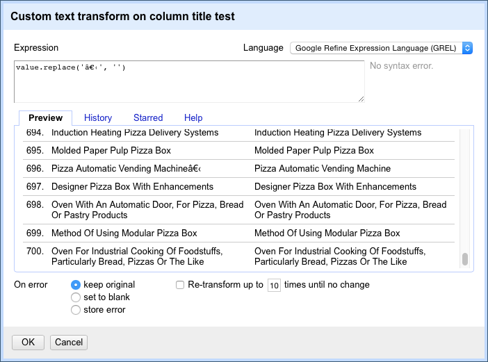
Chapter 8 Open Refine
Cleaning patent data is one of the most challenging and time consuming tasks involved in patent analysis. In this chapter we will cover.
- Basic data cleaning using Open Refine
- Separating a patent dataset on applicant names and cleaning the names.
- Exporting a dataset from Open Refine at different stages in the cleaning process.
Open Refine is an open source tool for working with all types of messy data. It started life as Google Refine but has since migrated to Open Refine. It is a programme that runs in a browser on your computer but does not require an internet connection. It is a key tool in the open source patent analysis tool kit and includes extensions and the use of custom code for particular custom tasks. In this article we will cover some of the basics that are most relevant to patent analysis and then move on to more detailed work to clean patent applicant names.
The reason that patent analysts should use Open Refine is that it is the easiest to use and most efficient free tool for cleaning patent data without programming knowledge. It is far superior to attempting the same cleaning tasks in Excel or Open Office. The terminology that is used can take some getting used to, but it is possible to develop efficient workflows for cleaning and reshaping data using Open Refine and to create and reuse custom codes needed for specific tasks.
In this chapter we use Open Refine to clean up a raw dataset from WIPO Patentscope containing nearly 10,000 raw records that make some kind of reference to the word pizza in the whole text. To follow this chapter using one of our training sets, download it from the Github repository here or use your own dataset.
8.1 Install Open Refine
To install Open Refine visit the Open Refine website and download the software for your operating system:

From the download page select your operating system. Note the extensions towards the bottom of the page for future reference.
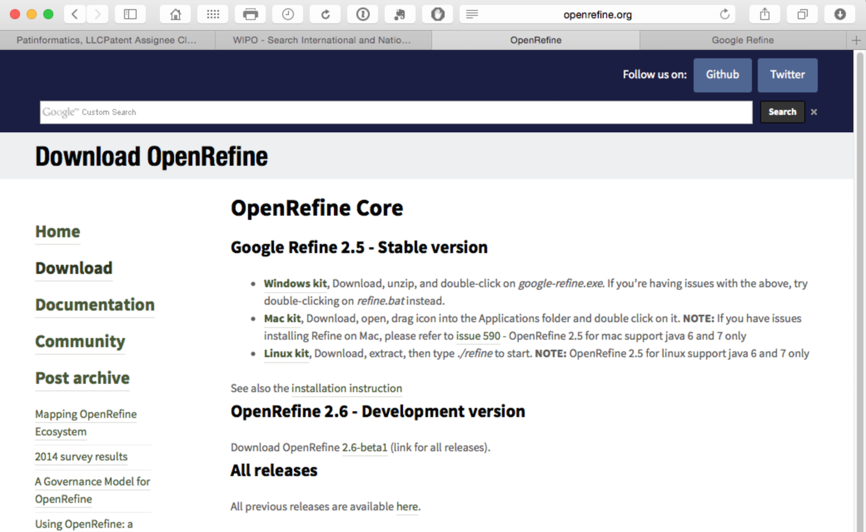
At the time of writing, when you download Open Refine it actually downloads and installs as Google Refine (reflecting its history) and so that is the application you will need to look for and open.
8.2 Create a Project
We will use the Patentscope Pizza Medium file that can be downloaded from the repository here.
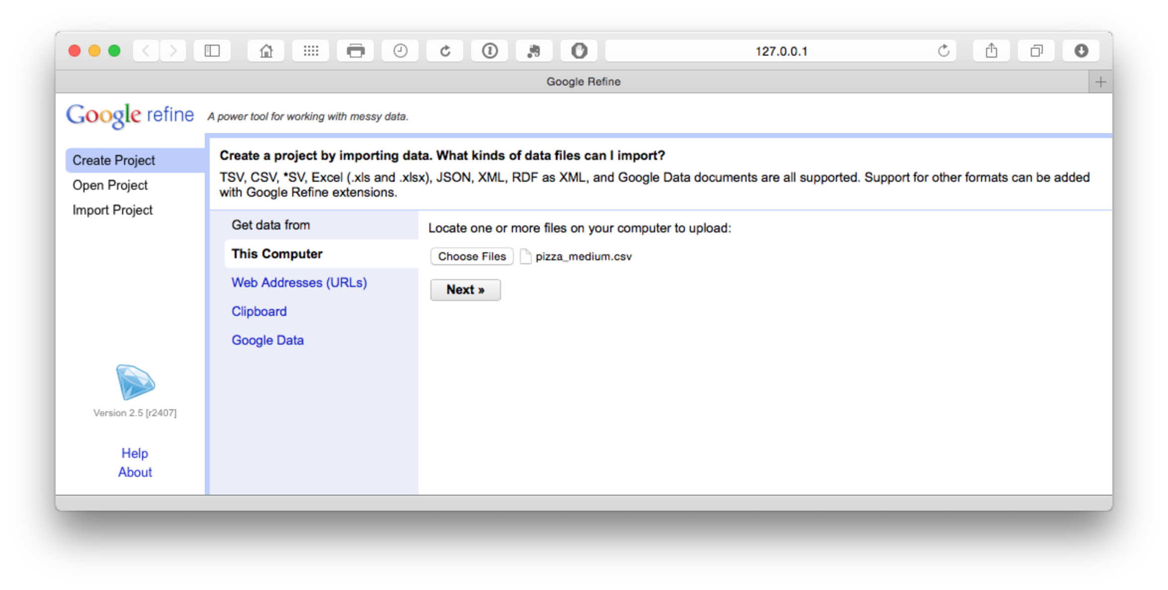
The file will load and then attempt to guess the column separator. Choose .csv. Note that a wide range of files can be imported and that there are additional options such as storing blank cells as nulls that are selected by default. In the dataset that you will load we have prefilled blank cells with NA values to avoid potential problems using fill down in Open Refine discussed below.
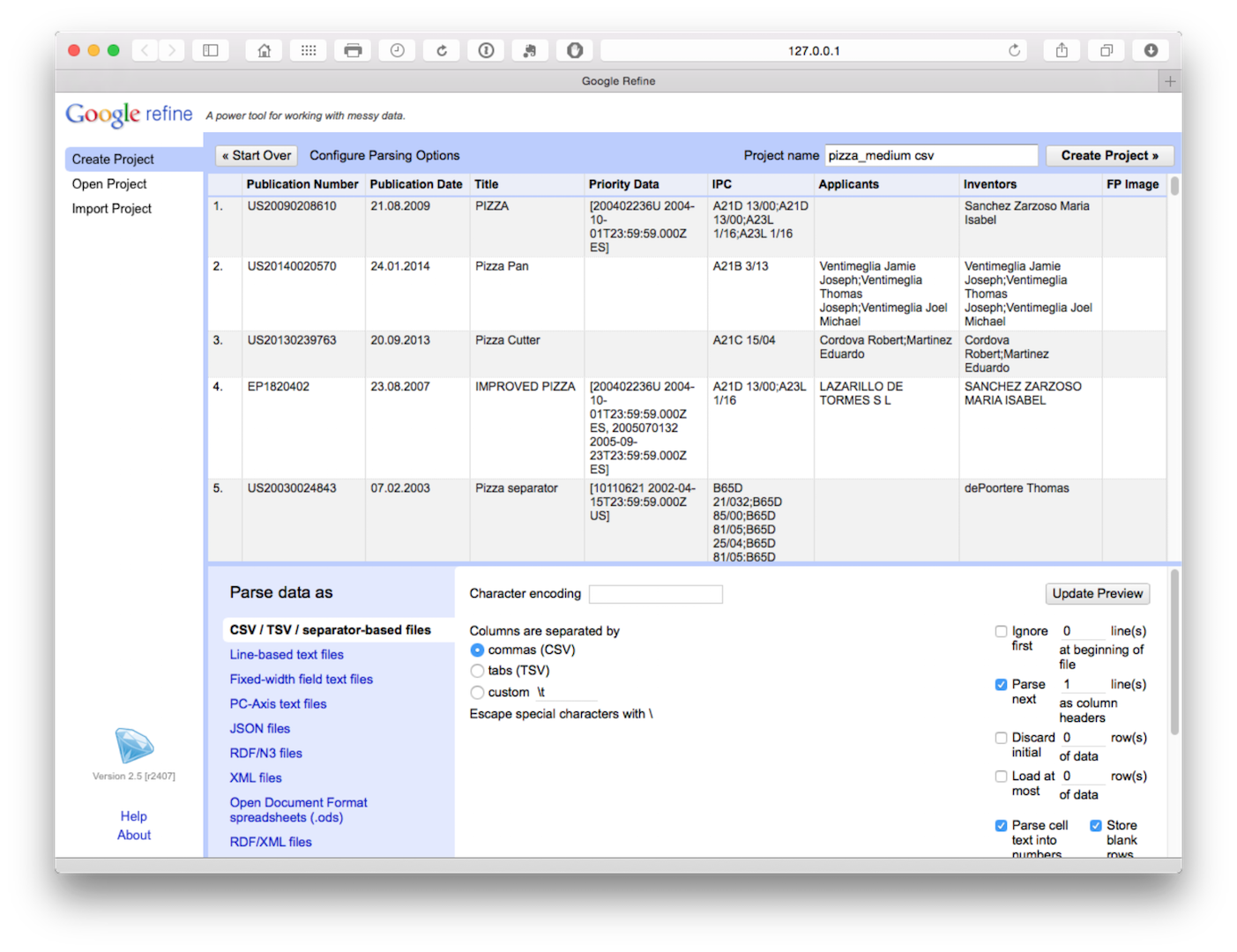
Click create project in the top right of the bar as the next step.
8.3 Open Refine Basics
A few basic features of Open Refine will soon have you working smoothly. Here is a quick tour.
8.3.1 Open Refine runs in a browser
Open Refine is an application that lives on your computer but runs in a browser. However, it does not require an internet connection and it does not lose your work if you close the browser.
8.3.2 Open Refine works on columns.
At the top of each column is a pull down menu. Be ready to use these menus quite a lot. In particular, you will often use the Edit cells > Common tranforms as shown below for functions such as trimming white space.
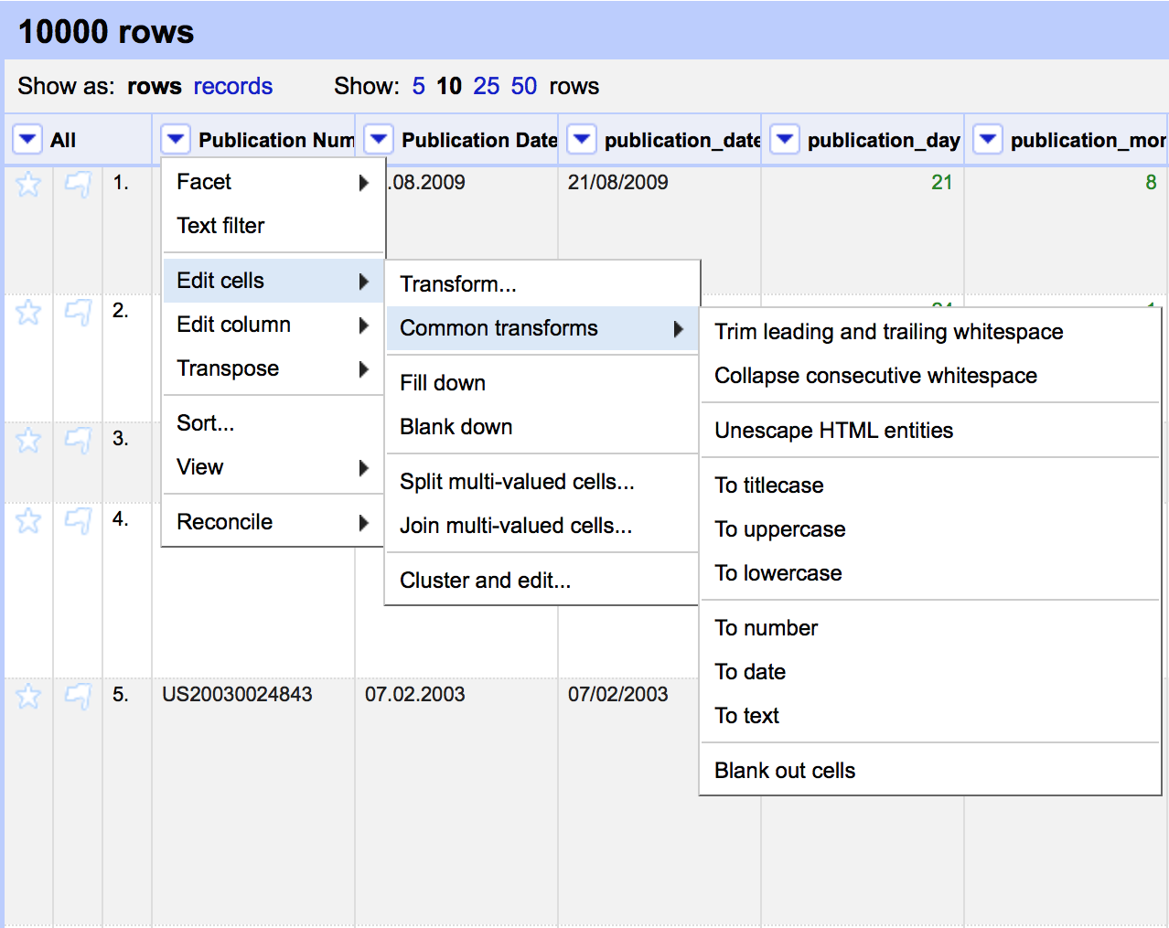
Other important menus are Edit column, immediately below Edit cells, for copying or splitting columns into new columns.
8.3.3 Open Refine works with Facets.
The term facet may initially be confusing but basically calls up a window that arranges the items in a column for inspection, sorting, and editing as we can see below. This is important because it becomes possible to identify problems and address them. It also becomes possible to apply a variety of clustering algorithms to clean up the data. Note that the size of the facet window can be adjusted by dragging the bottom of the window as we have done in this image.
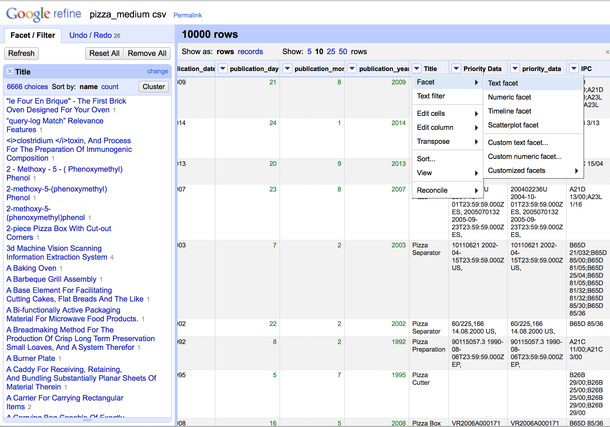
Hovering over an item inside the facet window brings up a small edit button that allows editing, such as removing and from the title.
8.3.4 Custom Facets
The Facet menu below brings up a custom menu with a range of options. Selecting Custom text facet (see below) brings up a pop up that allows for the use of code in Open Refine Expression Language (GREL) to perform tasks not covered by the main menu items. This language is quite simple and can range from short snippets for finding and replacing text to more complex functions that can be reused in future. We will demonstrate the use of this function below.

8.3.5 Reordering Columns
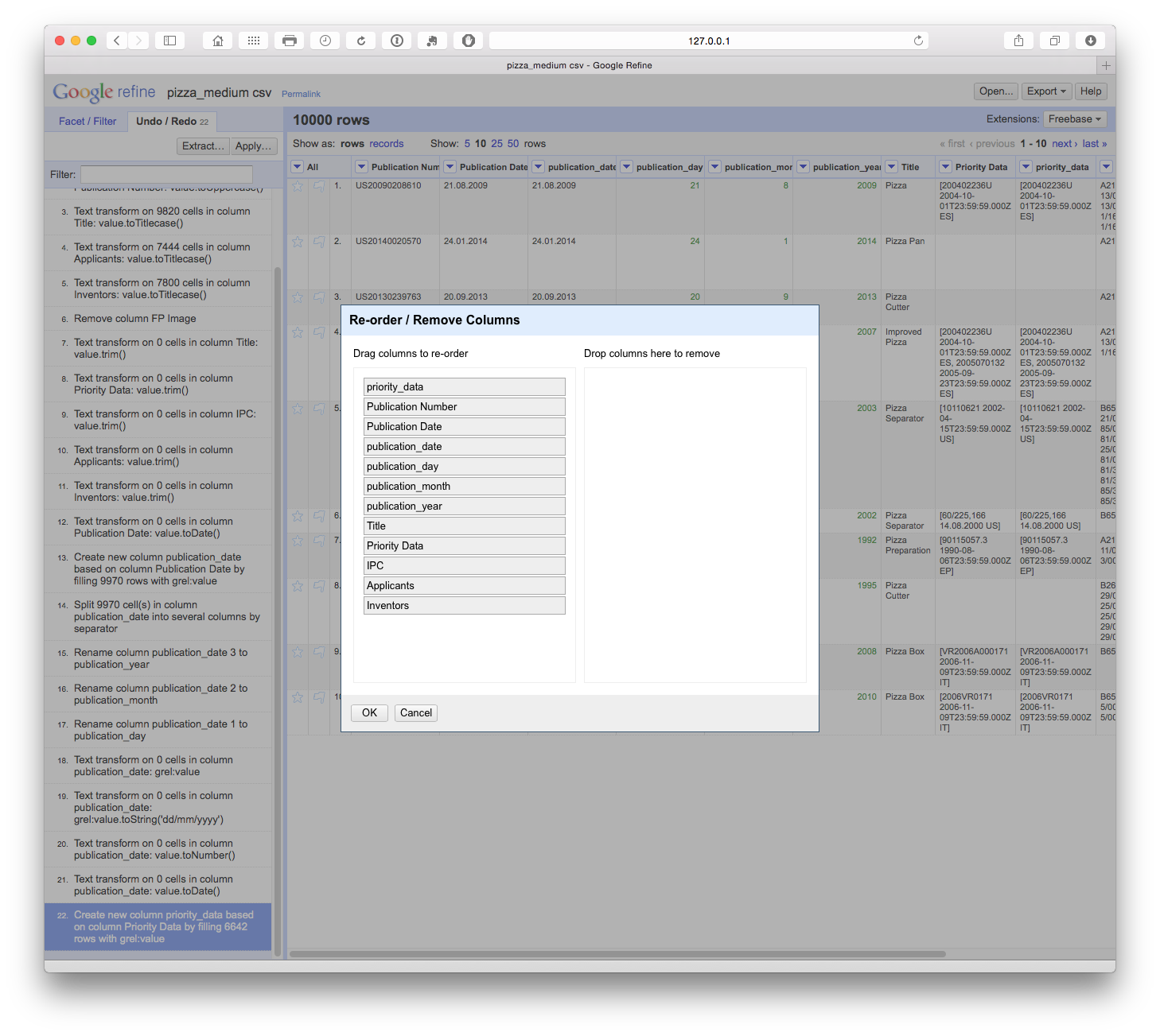
There are two options for reordering columns. The first is to select the column menu then Edit column > Move column to beginning. The second option, shown below, is to select the All drop down menu in the first column and then Edit columns > Re-order/remove columns. In the pop up menu of fields drag the desired field to the top of the list. In this case we have dragged the priority_date column to the top of the list. It will now appear as the first data column.
8.3.6 Undo and Redo
Open Refine keeps track of each action and allows you to go back several steps or to the beginning. This is particularly helpful when testing whether a particular approach to cleaning (e.g. splitting columns or using a snippet of code) will meet your needs. In particular it means you can explore and test approaches while not worrying about losing your previous work.
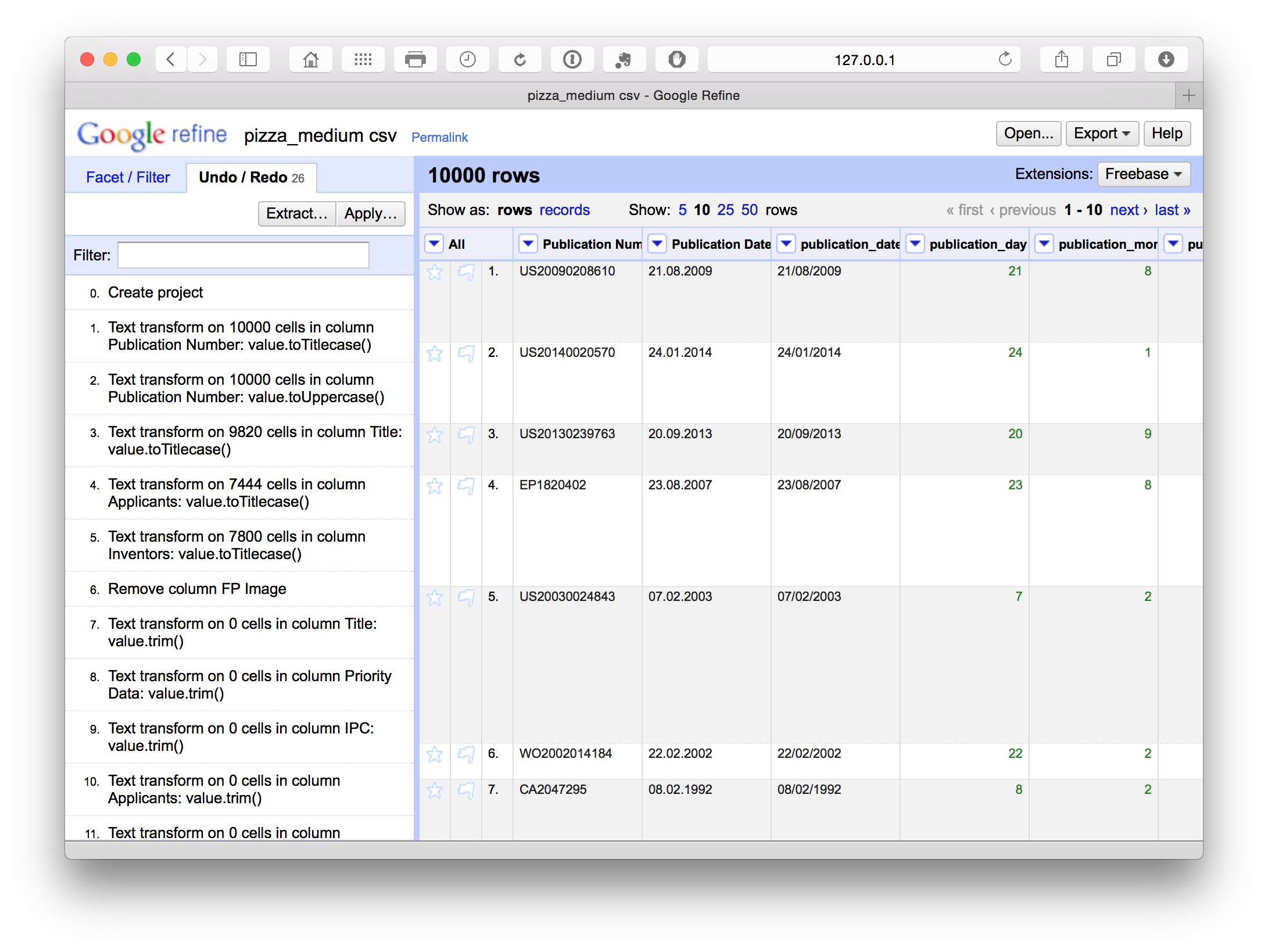
However, it can be important to plan the steps in your clean up operation to avoid problems at later stages. It may help to use a notepad as a checklist (see below). The main issue that can arise is where cleanup moves forward several steps without being fully completed in an earlier step. In some cases this can require returning to that earlier step, restarting and repeating earlier steps. As you become more familiar with Open Refine it will be easier to work out an appropriate sequence for your workflow.
8.3.7 Exporting
When a clean up exercise is completed a file can be exported in a variety for formats. When working with patent data expect to create more than one file (e.g. core, applicants, inventors, IPC) to allow for analysis of aspects of the data in other tools. In this chapter we will create two files.
- A cleaned version of the original data
- An applicants file that separates the data by each applicant.
8.4 Basic Cleaning
This is the first step in working with a dataset and it will make sense to perform some basic cleaning tasks before going any further. The Pizza Medium dataset that we are working with in this article is raw in the sense that the only cleaning so far has been to remove the two empty rows at the head of the data table and to fill blank cells with NA values. The reason that it makes sense to do some basic cleaning before working with applicant, inventor or IPC data is that new datasets will be generated by this process.
Bear in mind that Open Refine is not the fastest programme and make sure that you allocate sufficient time for the clean up tasks and are prepared to be patient while the programme runs algorithms to process the data. Note that Open Refine will save your work and you can return to it later.
When working with Open Refine we will typically be working on one column at a time. However, the key checklist for cleaning steps is:
- Make sure you have a back up of the original file. Creating a
.zipfile and marking it with the namerawcan help to preserve the original. - Open and save a text file as a
code bookto write down the steps taken in cleaning the data (e.g. pizza_codebook.txt). - Regularise characters (e.g. title, lowercase, uppercase).
- Remove leading and trailing white space.
- Address encoding and related problems.
Additional actions:
- Transform dates
- Access additional information and create new columns and/or rows.
We will generally approach these tasks in each column and steps 6 and 7 will not always apply. The creation of a codebook will allow you to keep a note of all the steps taken to clean up a dataset. The codebook should be saved with the cleaned dataset (e.g. in the same folder) as a reference point if you need to do further work or if colleagues want to understand the transformation steps.
8.4.1 Changing case
The first column in our Patentscope pizza dataset is the publication number. To inspect what is happening and needs to be cleaned in this column we will first select the column menu and choose text facet from the dropdown. This will generate the side menu panel that we can see below containing the data. We can then inspect the column for problems.
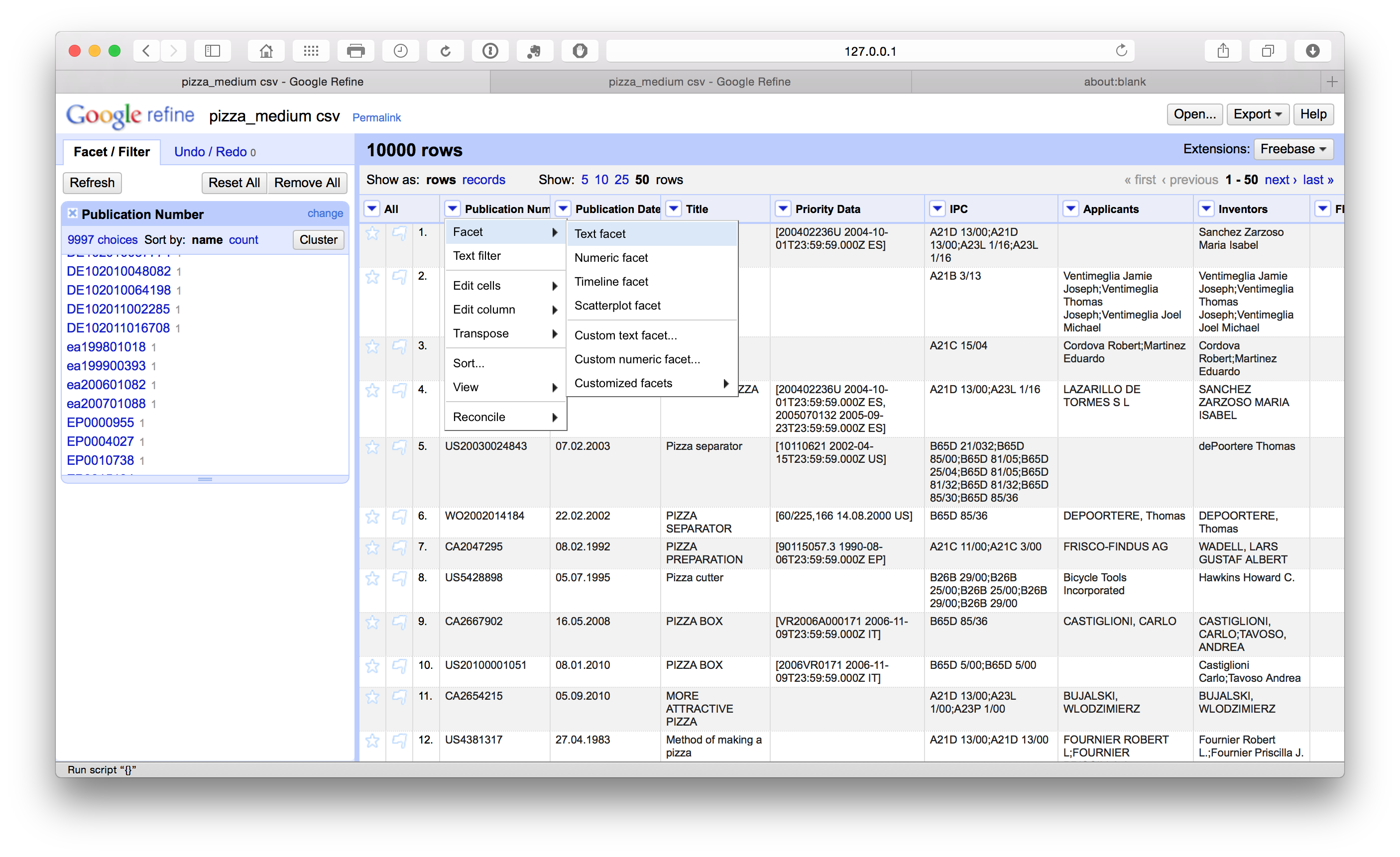
When we scroll down the side panel we can see that some publication numbers have a lowercase country code (in this case ea rather than EA for Eurasian Patent Organization using the WIPO standardized country codes). To address this we select the column menu Edit cells > Common transforms > to Uppercase.
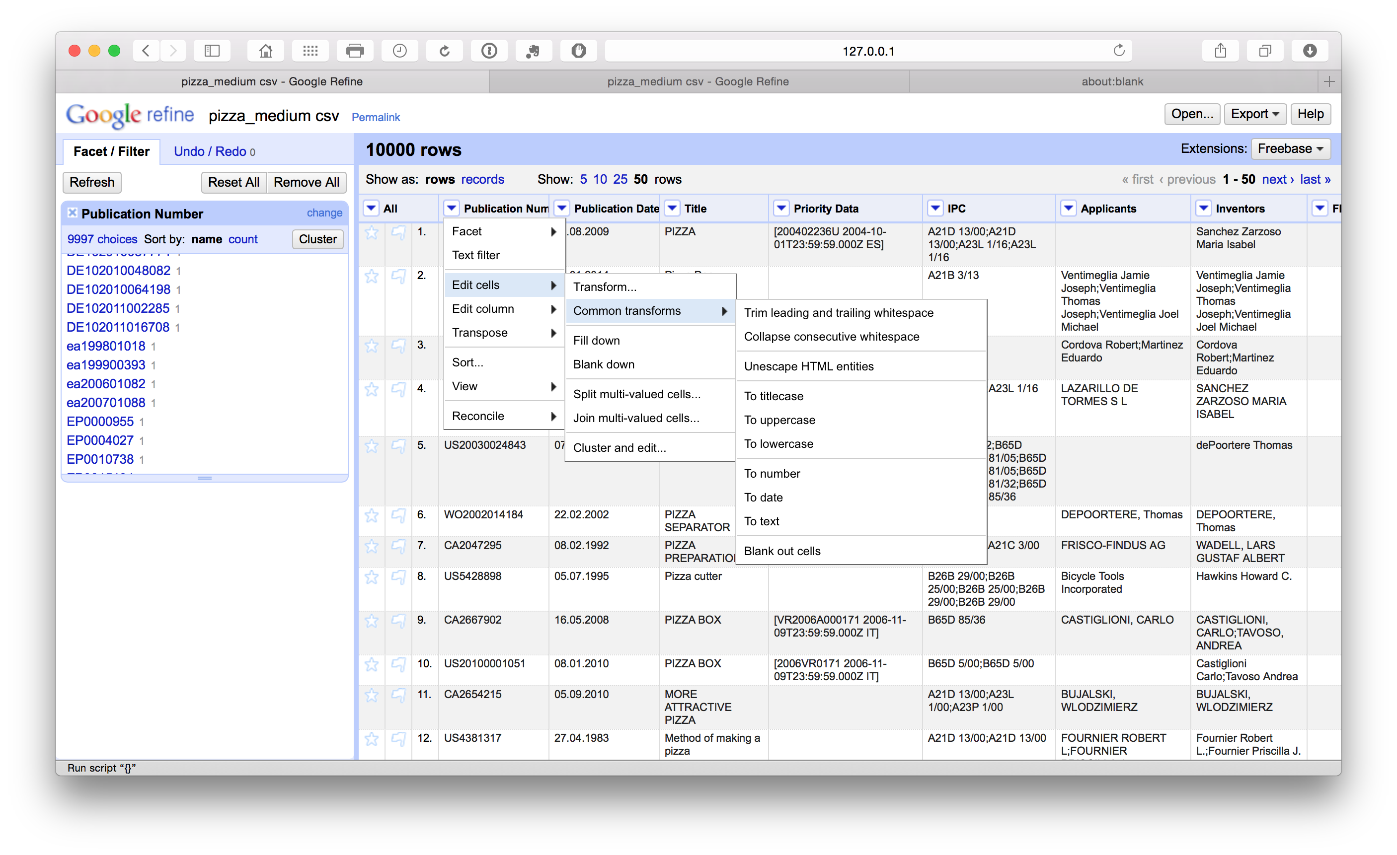
If we scroll down all the publication numbers will have been converted to upper case. This will make it easier to extract the publication country codes at a later stage.
8.4.2 Regularise case
For the other text columns it is sensible to repeat the common transformations step and select to titlecase. Note that this will generally work well for the title field but may not always work as well on concatenated fields such as applicants and inventor names. Repeat this step following the separation of these concatenated fields (see below on applicants). If the abstract or claims were present we would not regularise those text fields.
8.4.3 Remove leading and trailing whitespace
To remove leading and trailing white space in a column we select Edit cells > Common transforms > Trim leading and trailing white space across the columns.
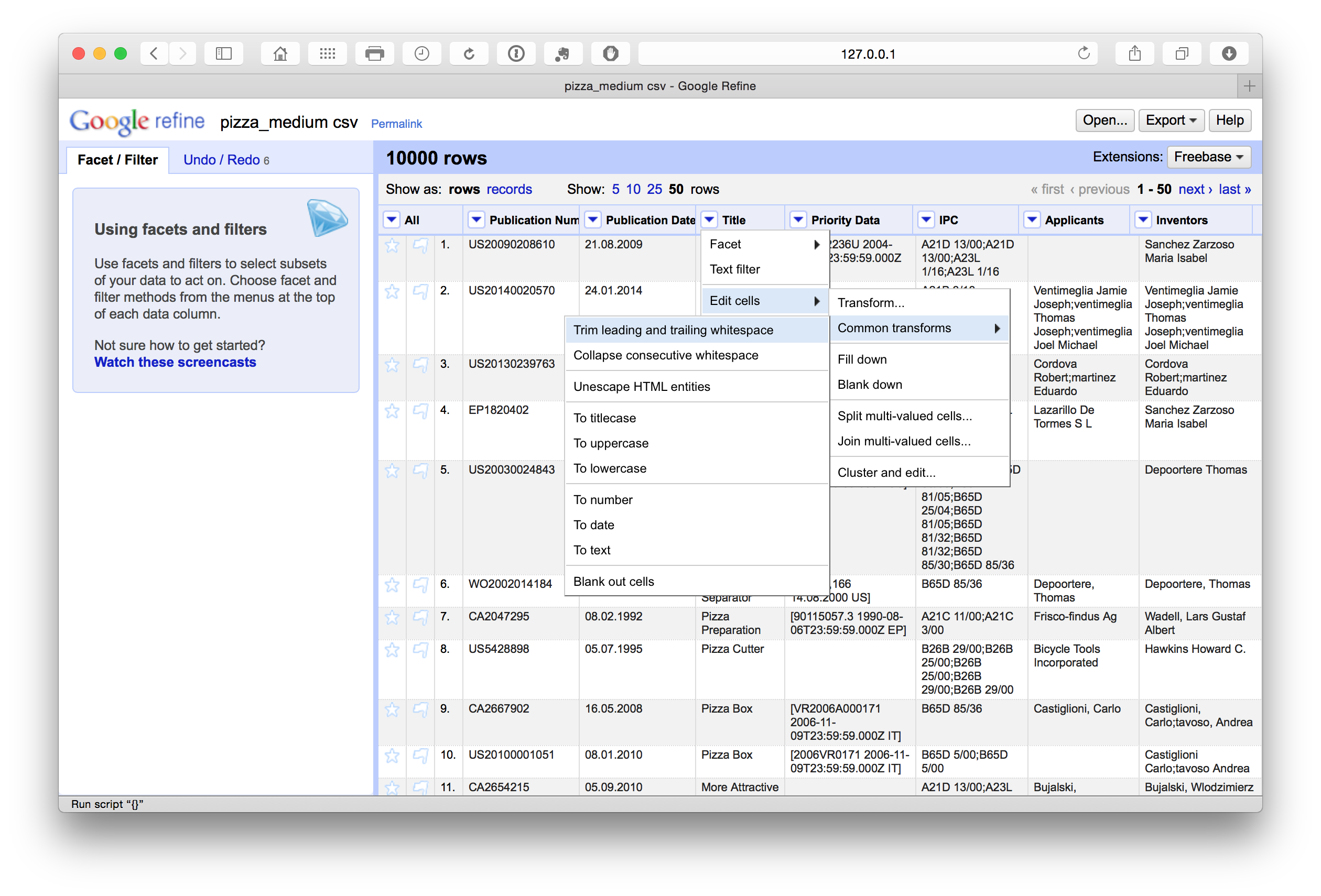
Note that following the splitting of concatenated cells with multiple entries such as the applicants and the inventors fields it is a good idea to repeat the trim exercise when the process is complete to avoid potential leading white space at the start of the new name entries.
8.4.4 Add Columns
We can also add columns by selecting the column menu and Edit Column > Add column based on this column. In this case we have added a column called publication_date.
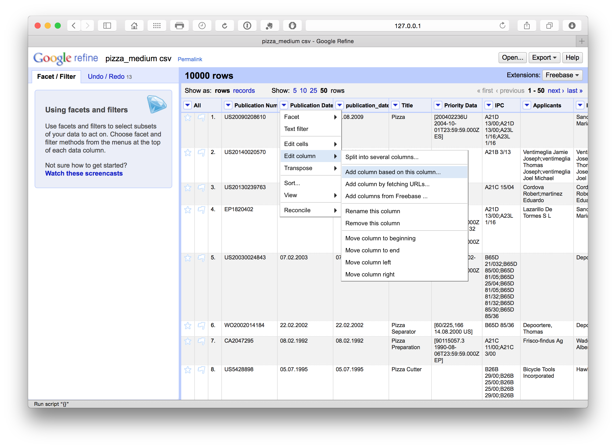
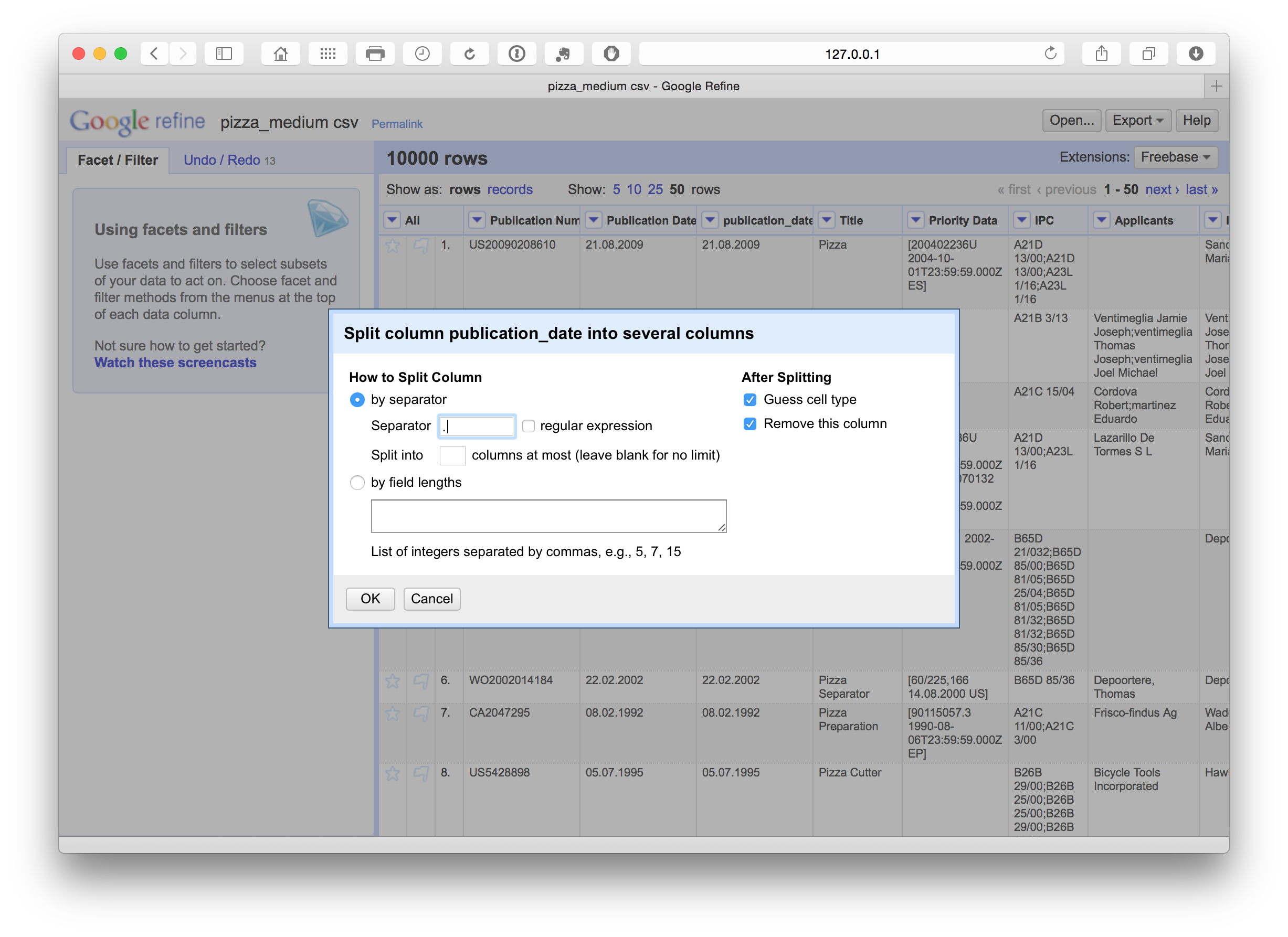
We have a number of options with respect to dates (see below). In this case we want to separate out the date information into separate columns. To do that we can use Edit column > Split into several columns. We can also choose the separator for the split, in this case . and whether to keep or delete the source column. In this case we selected to retain the original column and created three new date related columns. We could as necessary then delete the date and month column if we only needed the year field.
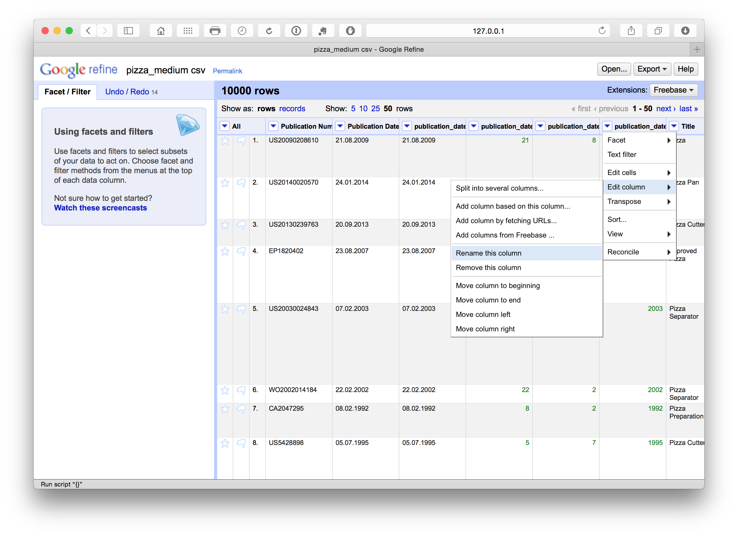
We can then rename these columns using the edit Edit Column > Rename this column. Note that in this case the use of lowercase and underscores marks out columns we are creating or editing as a flag for internal use informing us that this is a column that we have created. At a later stage we will rename the original fields to mark them as original.
8.4.6 Reformatting dates
One problem we may encounter is that the standard date definition on patent documents (e.g. 21.08.2009) may not be recognised as a date field in our analysis software because dates can be ambiguous from the perspective of software code. For example, how should 08/12/2009 or 12/08/2009 be interpreted?
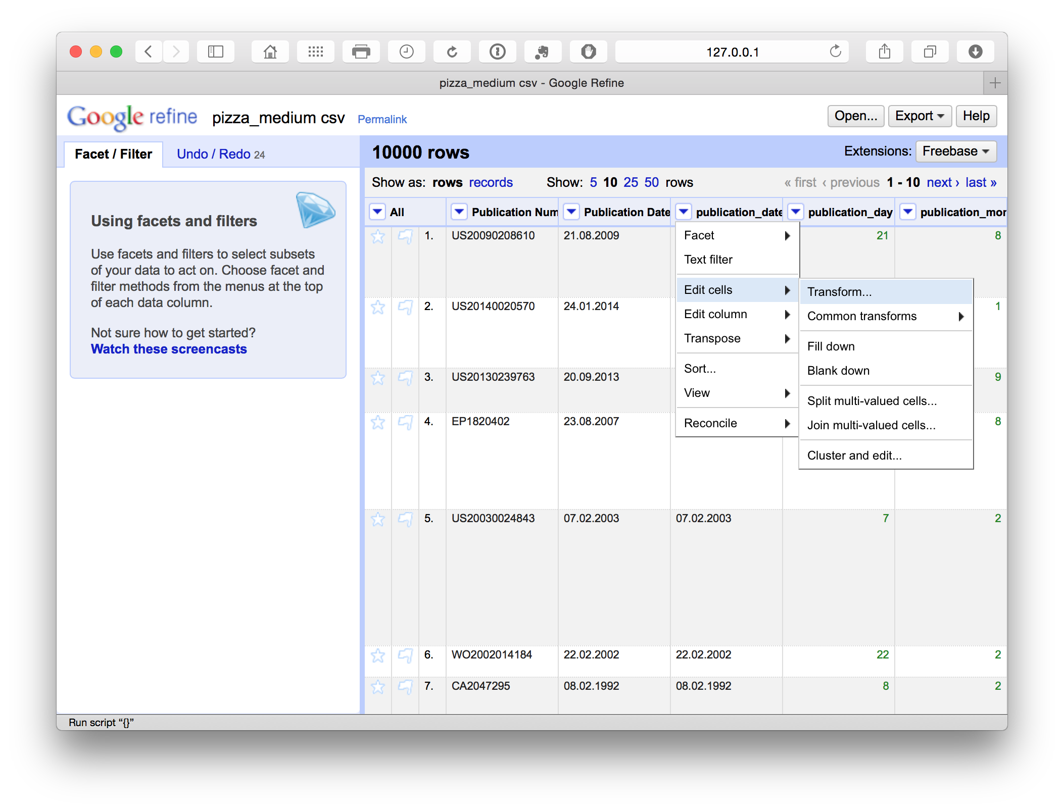
Alternatively, as in this case, the decimal points may not be correctly interpreted as signifying a date in some software (e.g. R). We might anticipate this and transform the data into a more recognisable form such as 21/08/2009. A very simple way to do this is by using a replace function. In this case we select the menu for the publication_date field and then Edit cells > Transform.
This produces a menu where we enter a simple GREL replace code.
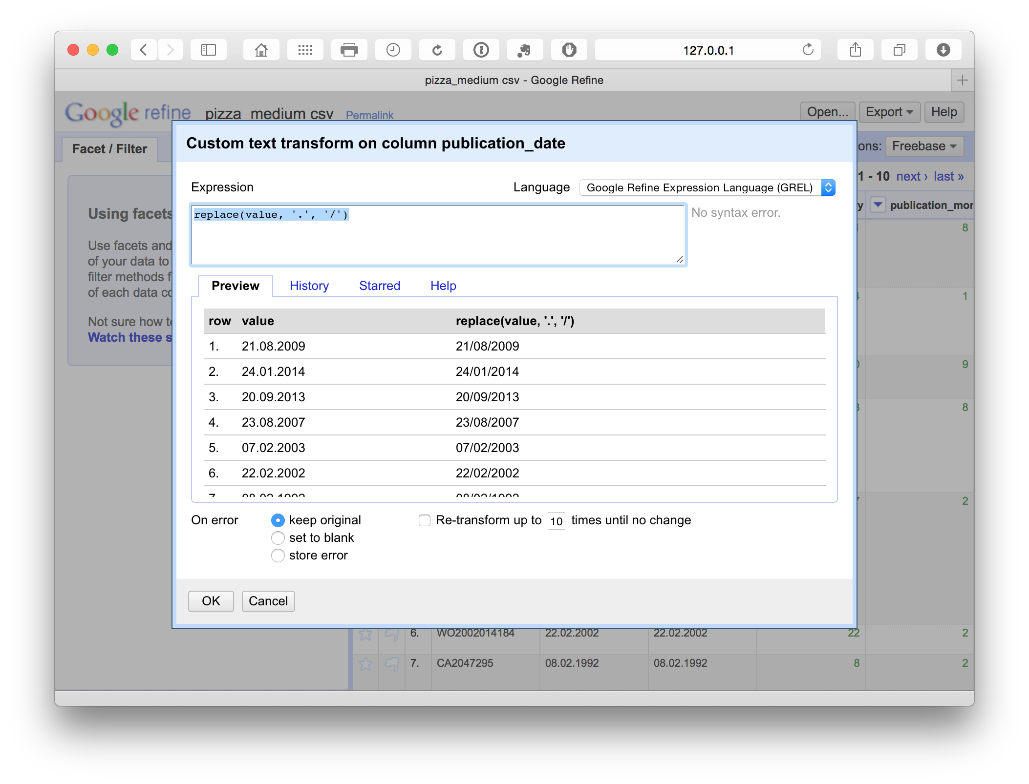
replace(value, '.', '/')This simple replace code is basically the same as find and replace in Excel or Open Office. In addition, we can see the consequences of the choice in the panel before we run the command. This is extremely useful for spotting problems. For example, if attempting to split a field on a comma we may discover that there are multiple commas in a cell (see the Priority Data field for this). By testing the code in the panel we could then work to find a solution or edit the offending texts in the main facet panel.
To find other simple codes visit the Open Refine Recipes page.
We will now focus on extracting information from some of the columns before saving the dataset and moving on.
8.4.7 Access additional information
There are a range of pieces of information that are hidden in data inside columns. For example, Patentscope data does not contain a publication country field. In particular, note that Patentscope merges all publications for an application record into one dossier. So we are only seeing one record for a set of documents (in Patentscope the wider dossier for a record is accessible through the Documents section of the website). This is very helpful in reducing duplication but it is important to bear in mind that we are not seeing the wider family in our data table. However, we can work with the information at the front of the publication number in the Patentscope records using a very simple code and create a new column (as above) based on the values returned as below.
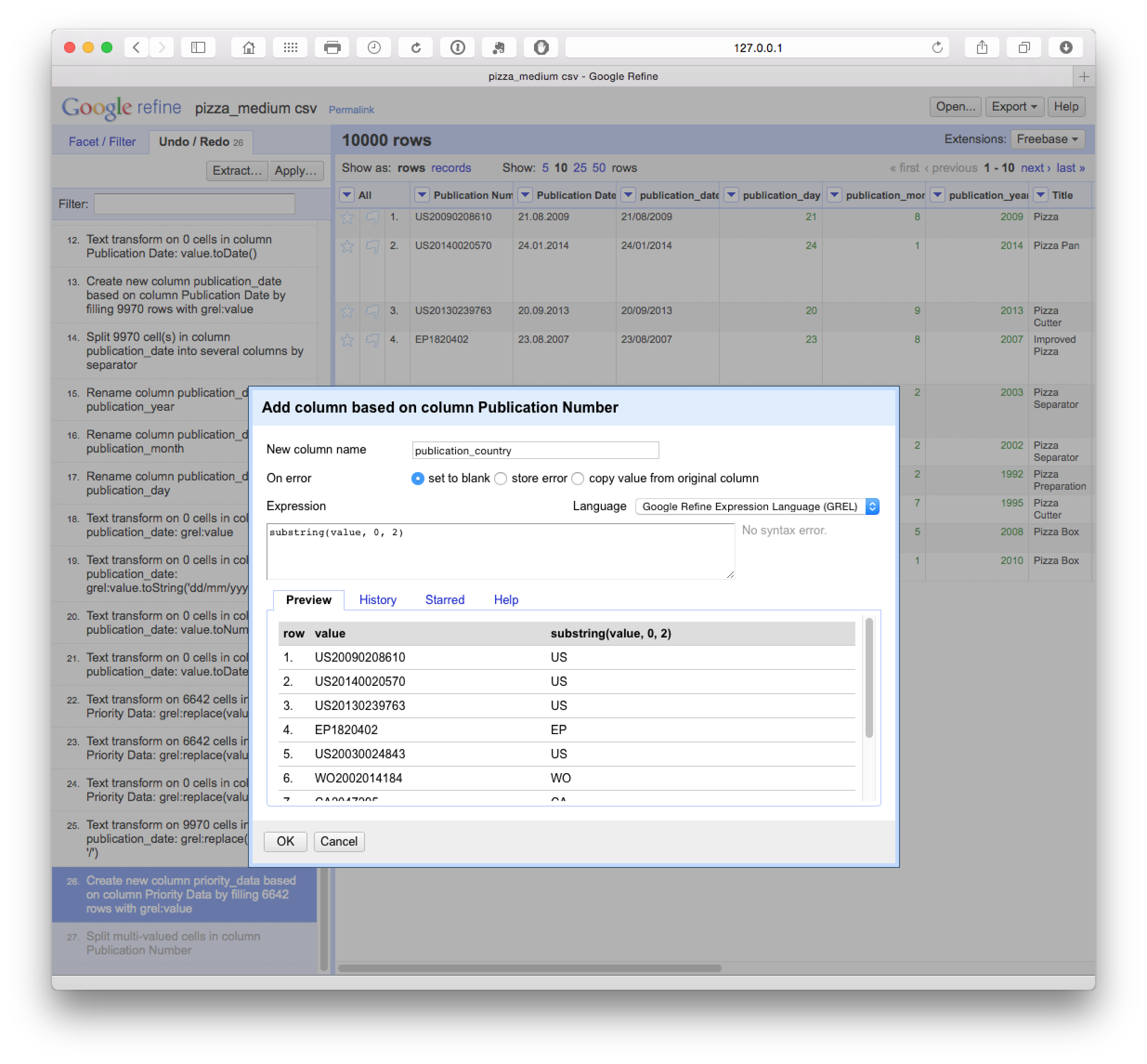
substring(value, 0, 2)Note here that the code begins counting from 0 (e.g. 0, 1 = U, 2 = S). The first part of the code looks in the value field. 0 tells the code to begin counting from 0 and the 2 tells it to read the two characters from 0. We could change these values, e.g to 1 and 4 to capture only a chunk of a number.
8.5 Fill blank cells
Filling blank cells with a value (NA for Not Available) to prevent calculation problems with analysis tools later can be performed by selecting each column, creating a text facet, scrolling down to the bottom of the facet choosing (blank), edit and then entering NA for the value.
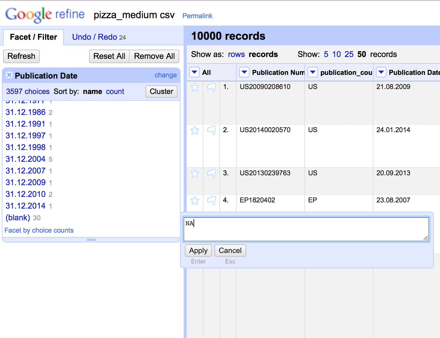
Note that this is somewhat time consuming (until a more rapid method is found) but has the benefit of being accurate. It is generally faster to open the file in Excel (or Open Office) and use find and replace with the find box left blank and NA in the replace field across the data table. For that reason, blank cells should not appear in the dataset you are using in this article. However, in later steps below we will be generating blank cells by splitting the applicant and inventor field. It is therefore important to know this procedure.
8.6 Renaming columns
At this stage we have a set of columns that are mixed between the original sentence case and the additions in lower case with no spaces such as publication_number. This is a matter of personal preference but it is generally a good idea to regularise the case of all columns to make them easy to remember. In this case we will also add the word original to the columns to distinguish between those created by cleaning the data and those we have created.
8.7 Exporting Data
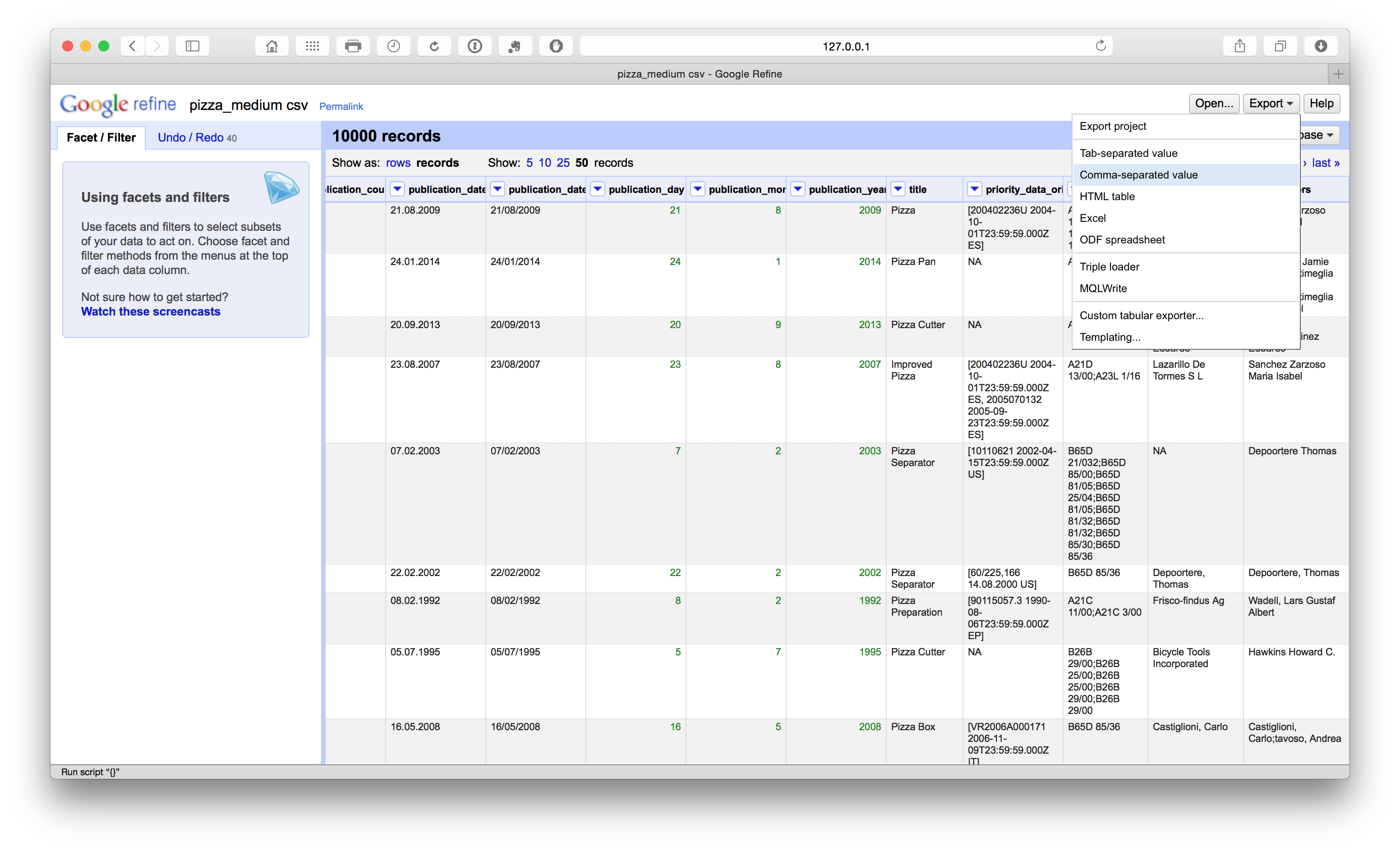
When we are happy that we have worked through the core cleaning steps it is a good idea to export the new core dataset. It is important to do this before the steps described below because it preserves a copy of the core dataset that can be used for separation (or splitting activities) on applicants, inventors, IPC etc. during the next steps. It is important that this clean dataset is as clean as is reasonably possible before moving on. The reason for this is that any noise or problems will multiply when we move on to the next steps. This may require a major rerun of the cleaning steps on later files created for applicants or inventors. Therefore make sure that you are happy that the data is as clean as is reasonably possible at this stage. Then choose export from the menu and the desired format (preferably .csv or .tab if using analytics tools later).
8.8 Splitting Applicants
This article was inspired by a very useful tutorial on cleaning assignee names with Google Refine by Anthony Trippe. Anthony is also the author of the forthcoming WIPO Guidelines for Preparing Patent Landscape Reports and the Patentinformatics LLC website has played a pioneering role in promoting patent analytics. We will take this example forward using the our sample pizza patent dataset so that it can be visualised in a range of tools. If you have not done so already, you can download the dataset here.
We actually have two options here and we will go through them so that you can work out your needs in a particular situation. Note that you can use Undo in Google Refine to go back to the point immediately before you tested these approaches. However, if you have followed the data cleaning steps above, make sure that you have already exported a copy of the main dataset.
8.8.1 Situation 1 - First Applicants
As discussed by Anthony Tripp we could split the applicant column into separate columns by choosing, Applicants > Edit column > Split into several columns.
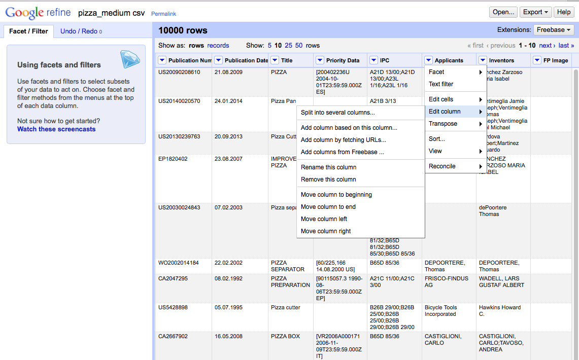
We then need to select the separator. In this case (and normally with patent data), it is ;.
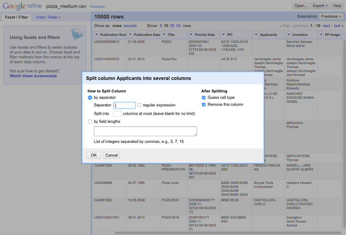
This will produce a set of 18 columns.
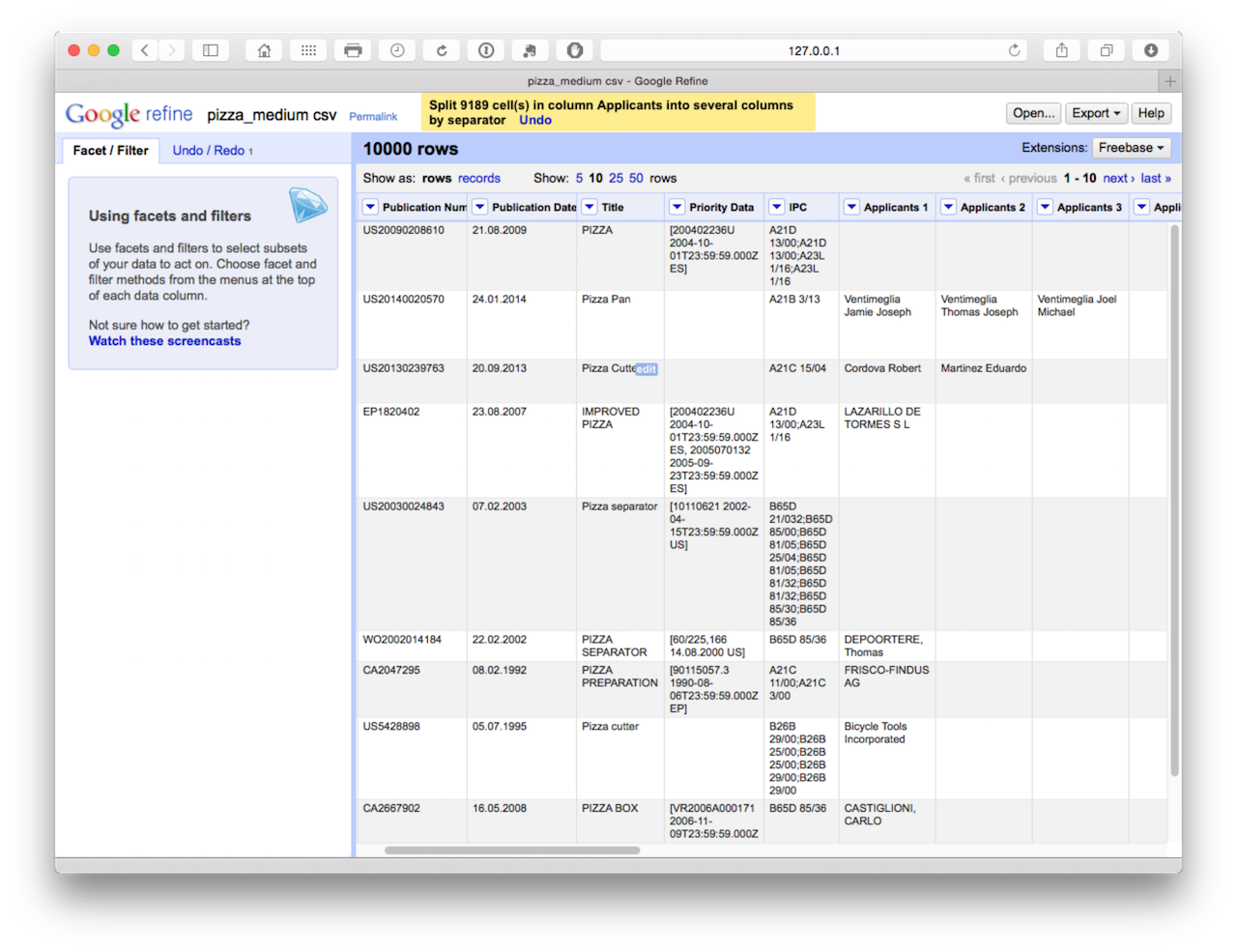
At this point, we could begin the clustering process to start cleaning the names that is discussed in situation 2. However, the disadvantage with this is that with this size of dataset we would need to do this 18 times in the absence of an easy way of combining the columns into a single column (applicants) with a name on each row. We might want to use this approach in circumstances where we are not focusing on the applicants and are happy to accept the first name in the list as the first applicant. In that case we would simply be reducing the applicant field to one applicant. Bear in mind that the first applicant listed in the series of names may not always be the first applicant as listed on an application and may not be an organisation name. Bearing these caveats in mind, we might also use this approach to reduce the concatenated inventors field to one inventor. For general purposes that would be clean and simple for visualisation purposes.
However, if we wanted to perform detailed applicant analysis for an area of technology, we would need to adopt a different approach.
8.8.2 Situation 2 - All Applicants
One of the real strengths of Open Refine is that it is very easy to separate applicant and inventor names into individual rows. Instead of choosing Edit column we now choose Edit cells and then split multi-valued cells.
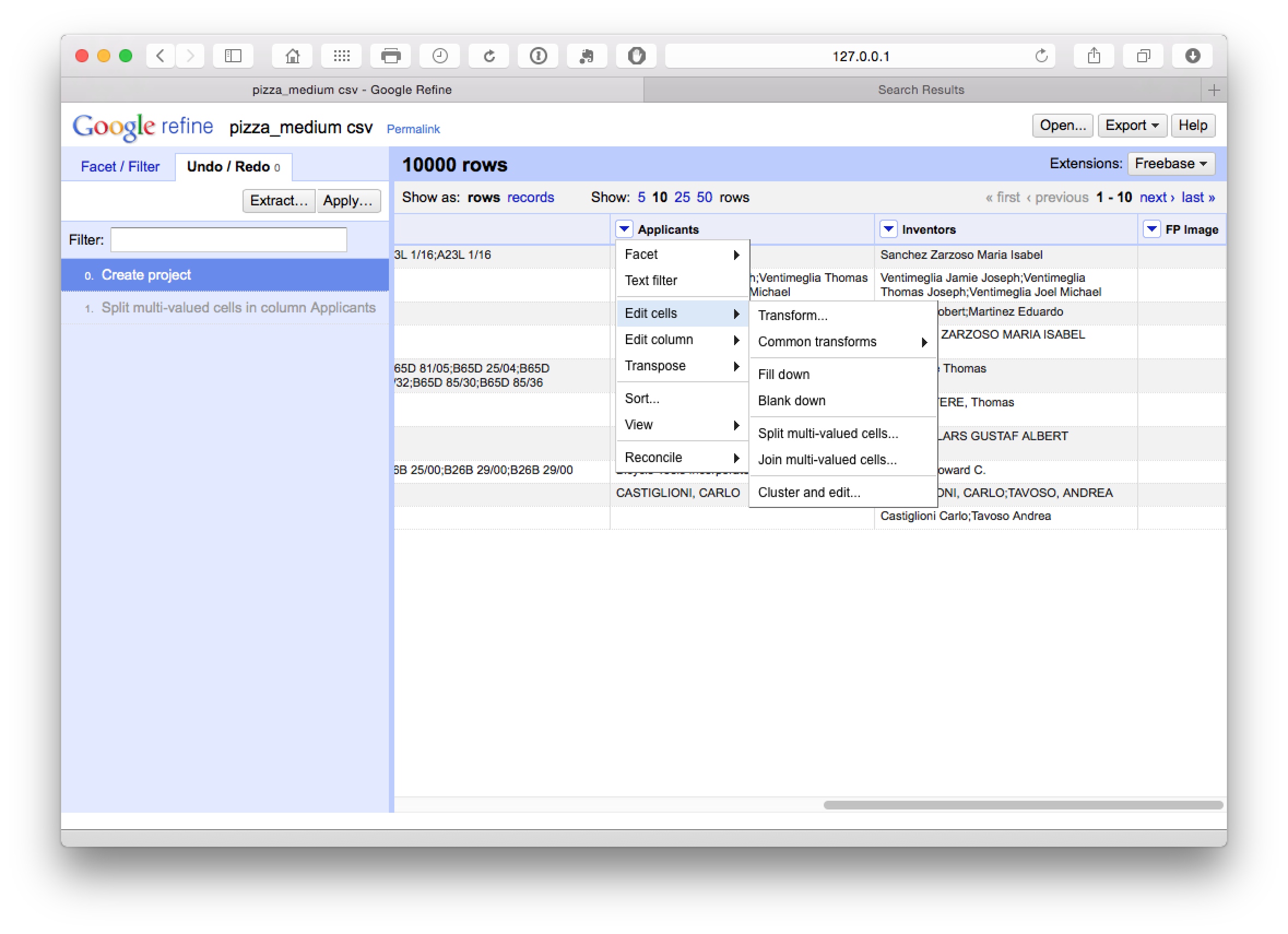
In the pop up menu choose ; as the separator rather than the default comma.
We now have a dataset with 15,884 rows as we can see below.
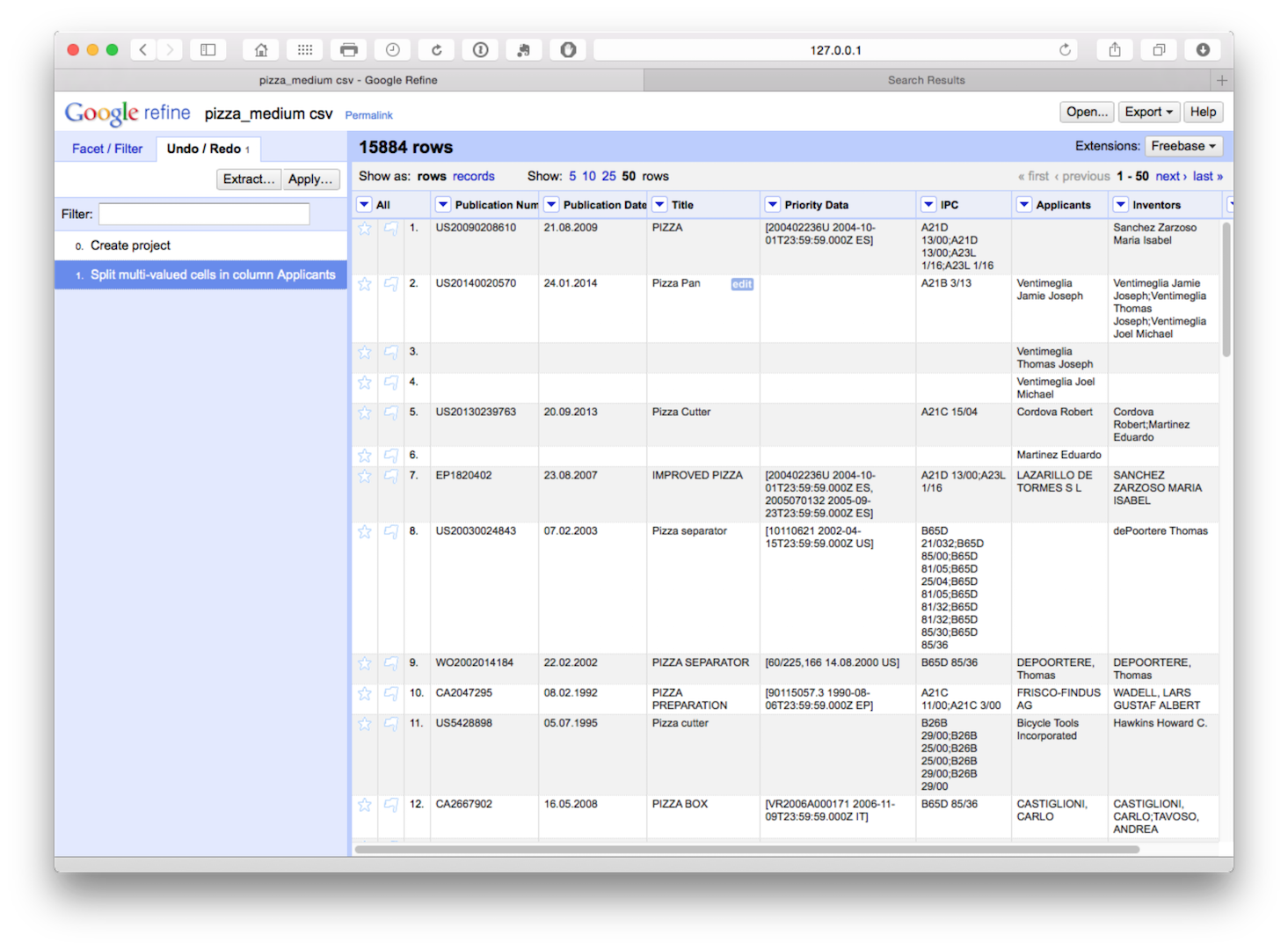
The advantage of this is that all our individual applicant names are now in a single column. However, note that the rest of the data has not been copied to the new rows. We will come back to this but as a precaution it is sensible to fill down on the publication number column as the key that links the individual applicants to the record. So let’s do that for peace of mind by selecting publication number > edit cells > fill down.
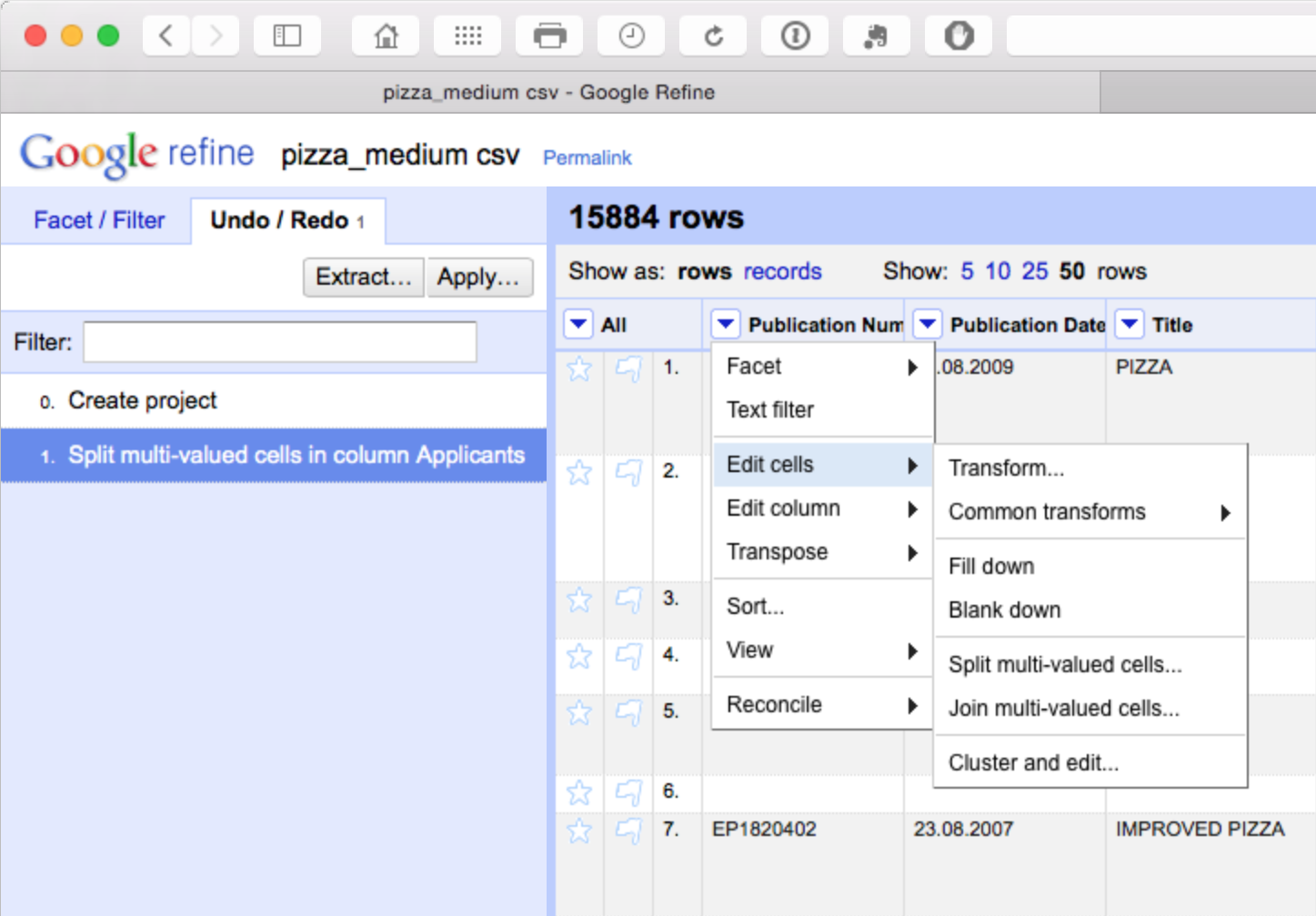
We should now have a column filled with the publication number values for each applicant as our key. Note here that there is a need for caution in using fill down in Open Refine as discussed in detail here. Basically, fill down is not performed by record, it simply fills down. That can mean that data becomes mixed up. This is another reason why it is important to fill blank values with NA either before starting work in Open Refine or as one of the initial clean up steps. Using NA early on will help prevent refine from filling down blank cells with the values of another record.
If you have not already done so above to assist the clean up process, and as general good practice, transform the mixed case in the applicants field to a single case type. To do that select Applicants > Edit Cells > Common Transformations > To titlecase.
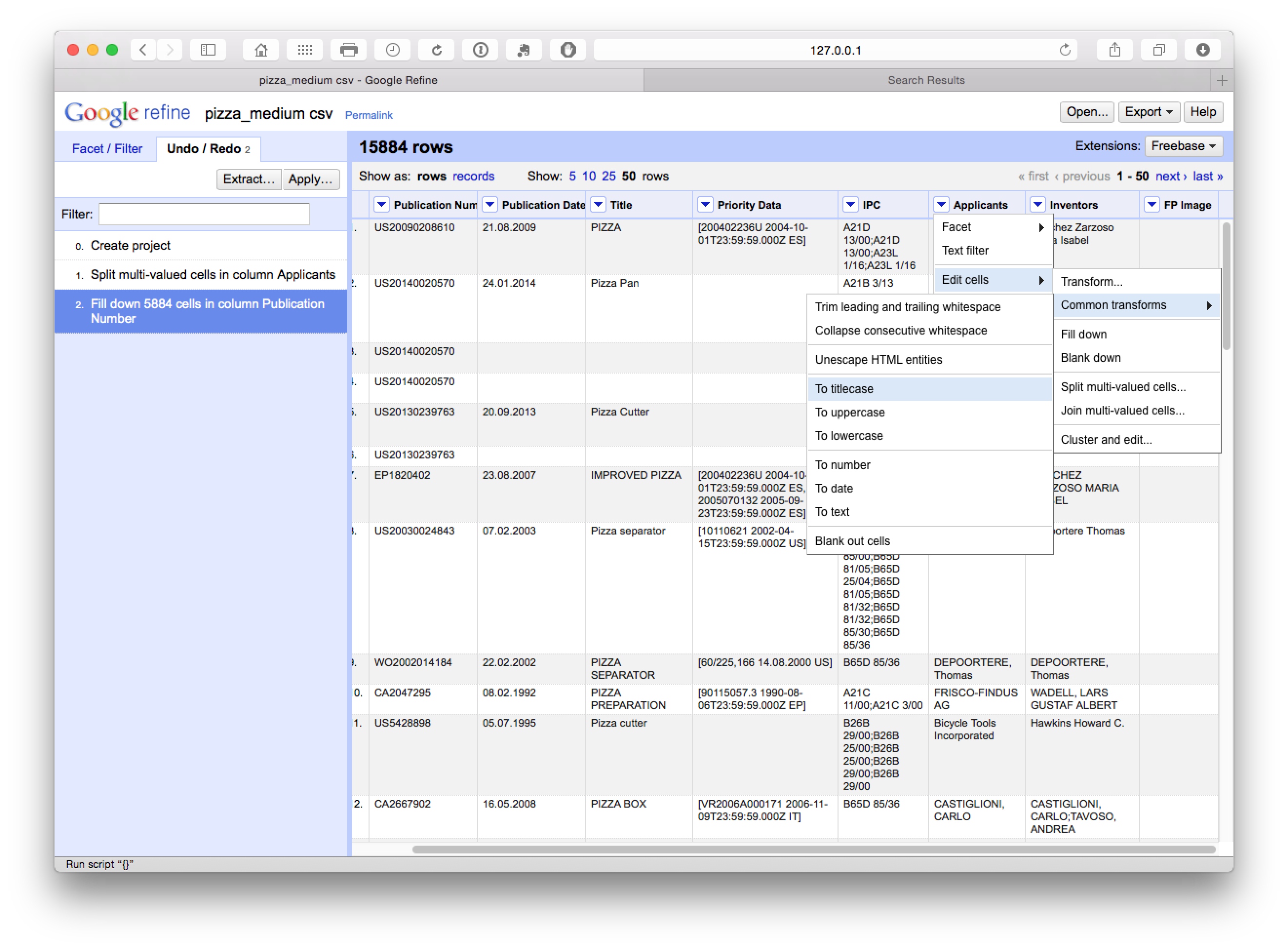
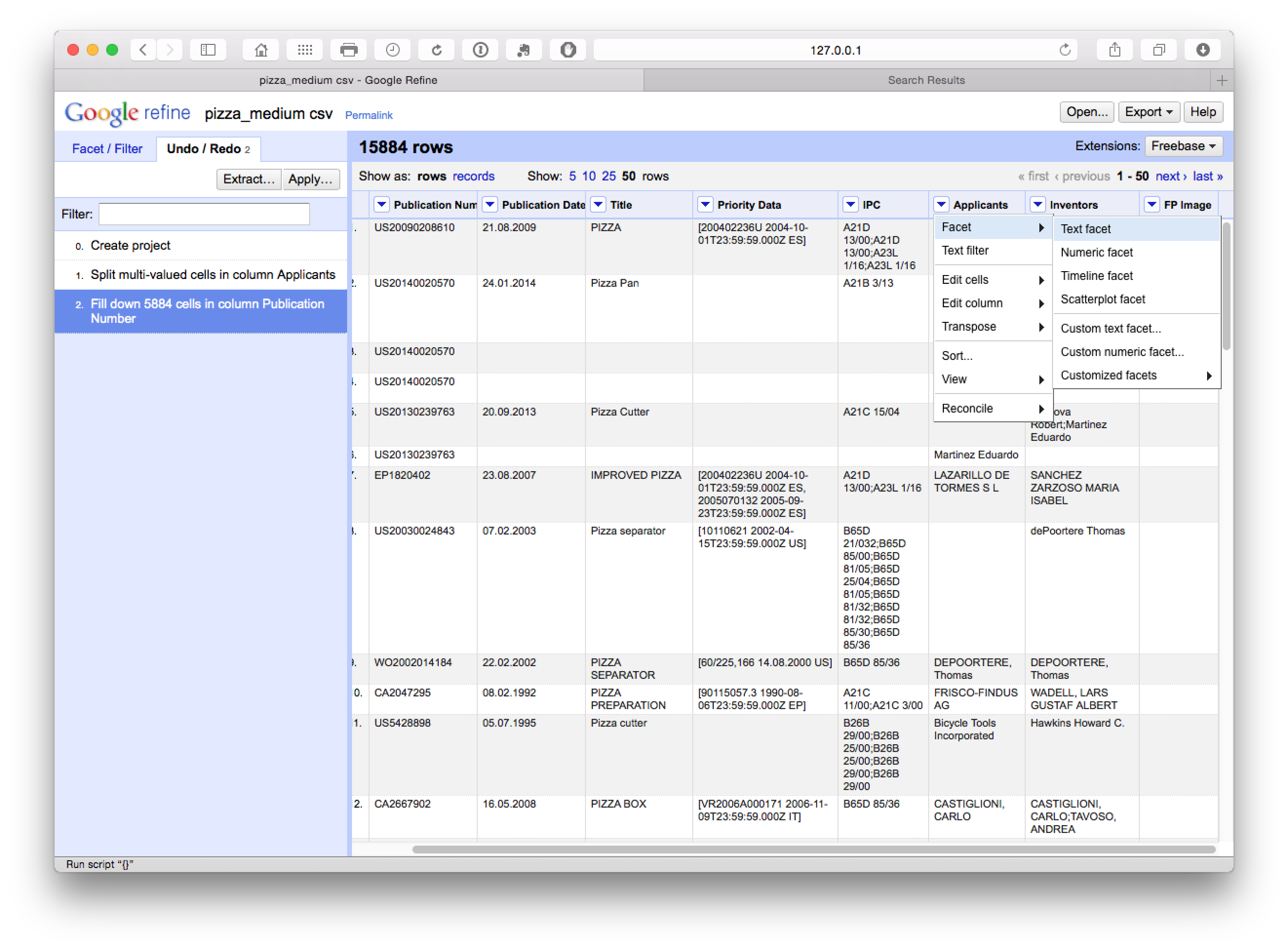
We now move back to the applicants and select Facet > Text Facet.
What we will see (with Applicants moved to the first column by selecting Applicants > Edit Column > Move column to beginning) is a new side window with 9,368 choices.
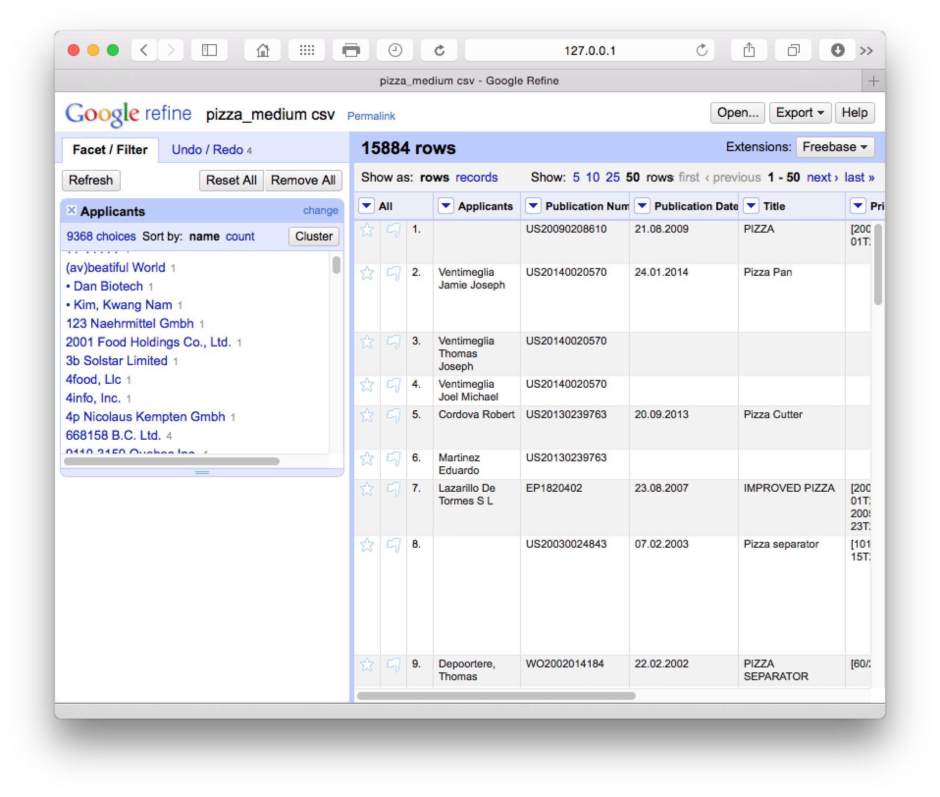
The cluster button will trigger a set of six clean up algorithms with user choices along the way. It is well worth reading the documentation on these steps to decide what will best fit your needs in future. These cleaning steps proceed from the strict to the lax in terms of matching criteria. The following is a brief summary of the details provided in the documentation page:
- Fingerprinting. This method is the least likely in the set to produce false positives (and that is particularly important for East Asian names in patent data). It involves a series of steps including removing trailing white space, using all lowercase, removing punctuation and control characters, splitting into tokens on white space, splitting and joining and normalising to ASCII.
- N-Gram Fingerprint. This is similar but uses n-grams (a sequence of characters or multiple sequences of characters) that are chunked, sorted and rejoined and normalised to ASCII text. The documentation highlights that this can produce more false positives but is food for finding clusters missed by fingerprinting.
- Phonetic Fingerprint. This transforms tokens into the way they are pronounced and produces different fingerprints to methods 2 & 3.
- Nearest Neighbour Methods. This is a distance method but can be very very slow.
- Levenshtein Distance. This famous algorithm measures the minimal number of edits that are required to change one string into another (and for this reason is widely known as edit distance). Typically, this will spot typological and spelling errors not spotted by the earlier approaches.
- PPM a particular use of Kolmogorov complexity as described in this article that is implemented in Open Refine as
Prediction by Partial Matching.
It is important to gain an insight into these methods because they may affect the results you receive. In particular, caution is required on East Asian names where cultural naming traditions produce a lot of false positive matches on the same name for persons who are actually distinct persons (synonyms or “lumping” in the literature). This can have very dramatic impacts on the results of patent analysis for inventor names because it will treat all persons sharing the name Smith, John or Wang, Wei as the same person, when in practice they are multiple individual people.
We will now walk through each algorithm to view the results.
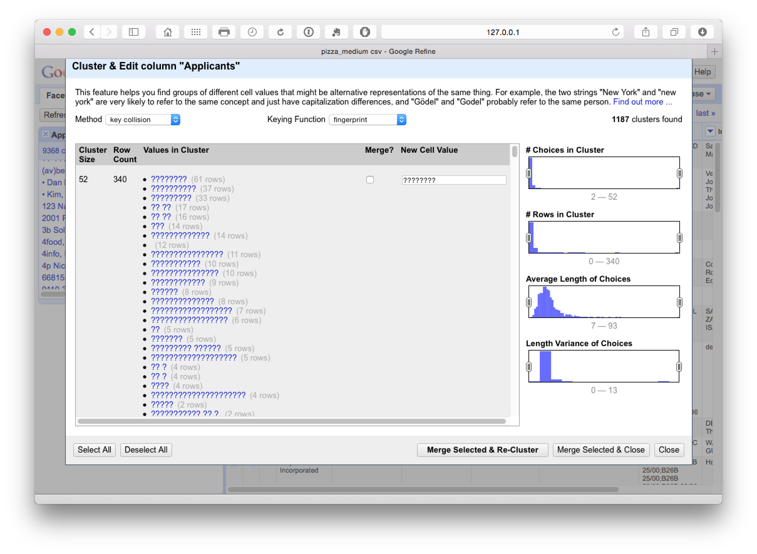
This identifies 1187 clusters dominated by hidden characters in the applicants field (typically appearing after the name). At this stage we need to make some decisions about whether or not to accept or reject the proposed merger by checking the Merge? boxes.
This step was particularly good at producing a match on variant names and name reversals as we can see here.
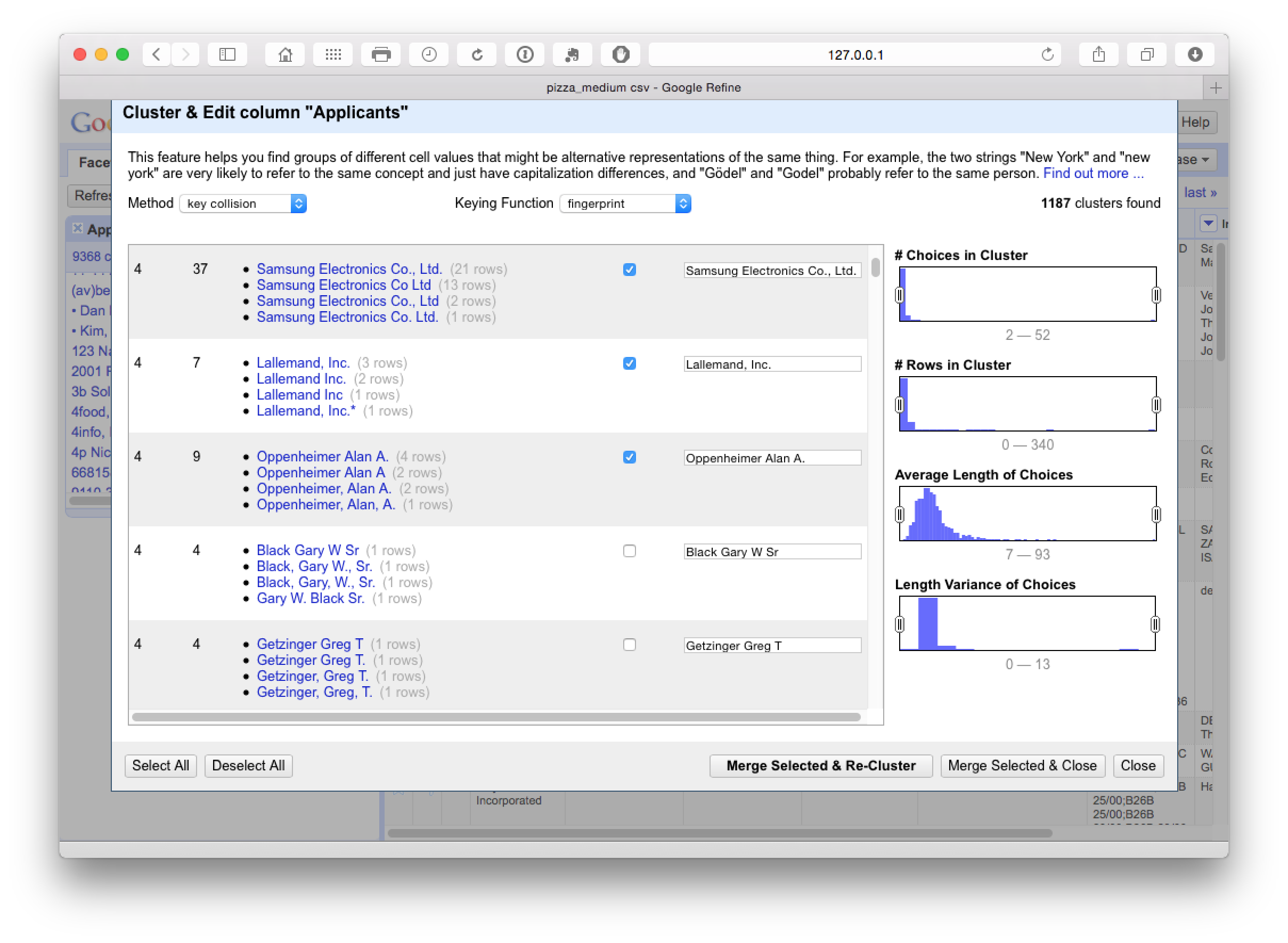
It pays to manually inspect the data before accepting it. One important option here is to use the slider on Choices in Cluster to move the range up or down and then make a decision about the appropriate cut off point. Then use select all in the bottom left for results you are happy with followed by Merge Selected & Re-Cluster. In the next step we can change the keying function dropdown to Ngram-fingerprint.
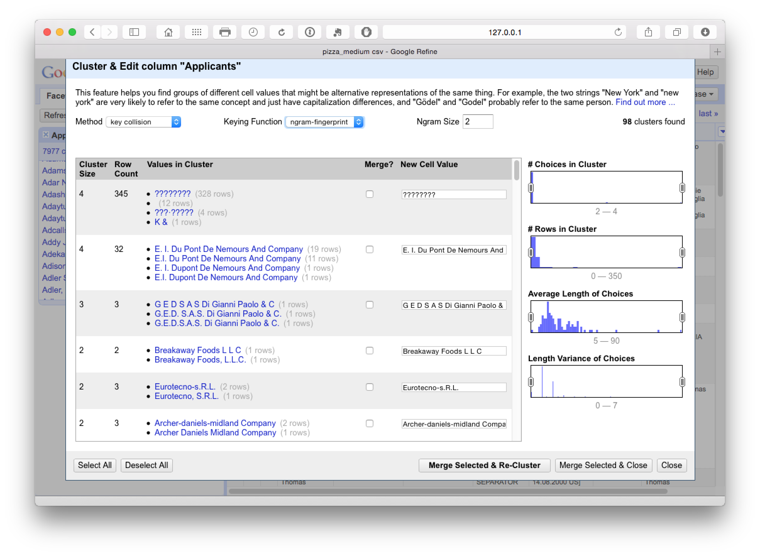
This produces 98 clusters which inspection suggests are very accurate. The issues to watch out for here (and throughout) are very similar names for companies that may not be the same company (such as Ltd. and Inc.) or distinct divisions of the same company. It is also important, when working with inventor names, not to assume that the same name is the same inventor in the absence of other match criteria, or that apparently minor variations in initials (e.g. Smith, John A and Smith, John B) are the same person because they may well not be.
To see these potential problems in action try reducing the N-gram size to 1. At this point we see the following.
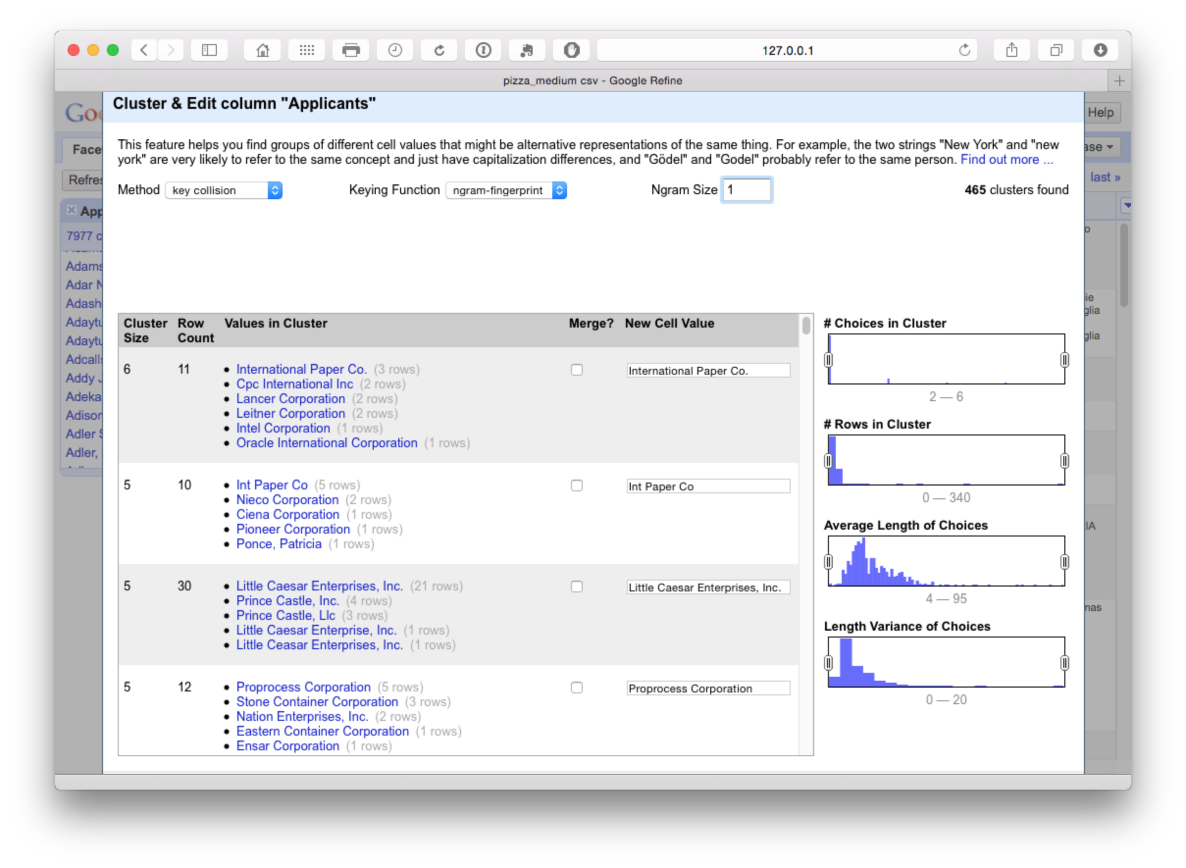
This measure is too lax and is grouping together companies that should not be grouped. In contrast increasing the N-gram value to 3 or 4 will tighten the cluster. We will select all on N-gram 2 and proceed to the next step.
At this point it is worth noting that the original 9,368 clusters have been reduced to 7,875 and if we sort on the count in the main window then Google is starting to emerge as the top applicant across our set of 10,000 records.
8.8.3 Phonetic Fingerprint (Metaphone 3) clustering
As we can see below, Metaphone 3 clustering produces 413 looser clusters with false positive matches on International Business Machines but positive matches on Cooperative Verkoop.
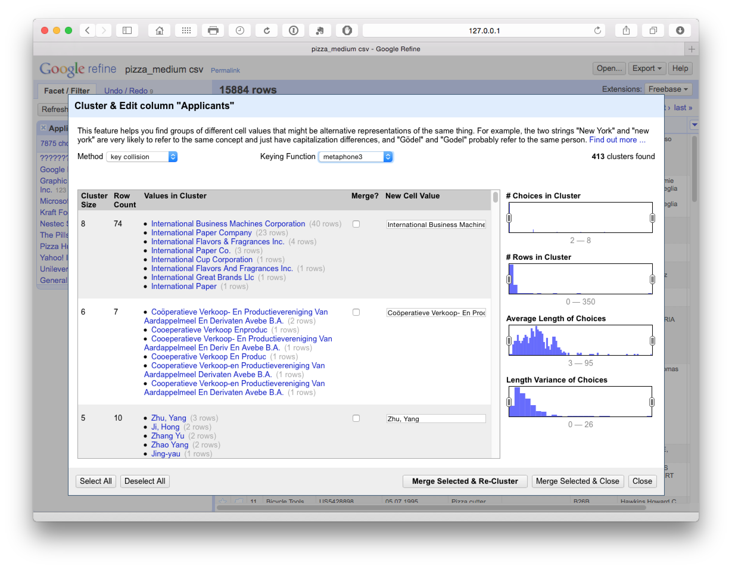
At this point we could either manually review the 413 clusters and select as appropriate or change the settings to reduce the number of clusters using the Choices in Clusters slider until we see something manageable for manual review. At this stage we might also want to use the browse this cluster function that appears on hovering over a particular selection, to review the data (see the second entry in the image below).
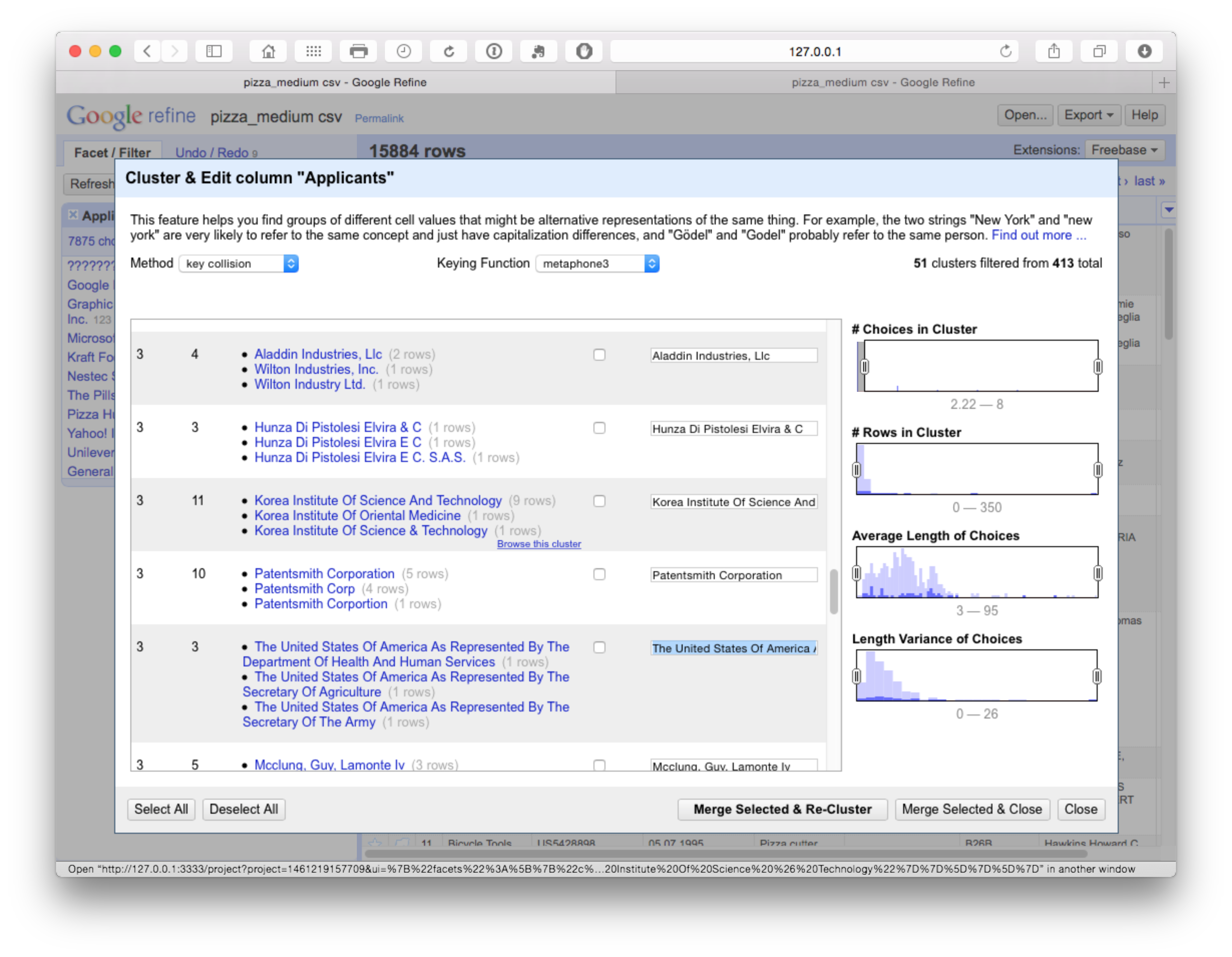
In this case we are attempting to ascertain whether the Korea Institute of Oriental Medicine should be grouped with the Korea Institute of Science and Technology (which appears unlikely). If we open the browser function we can review the entries for shared characteristics as possible match criteria.
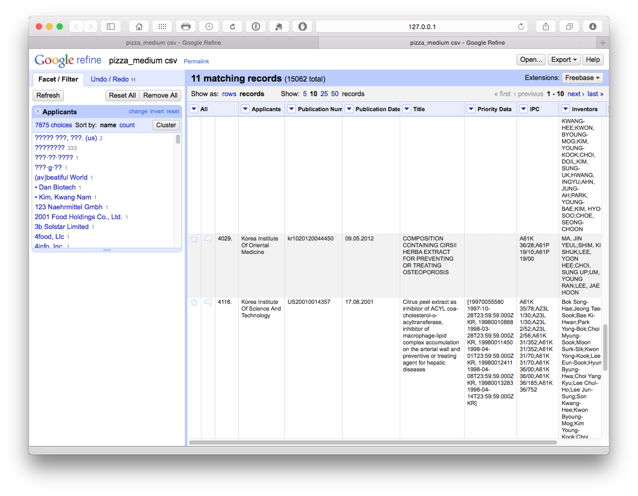
For example, if the applicants shared inventors and/or the same title we may want to record this record in the larger grouping (remembering that we have exported the original cleaned up data). Or, as is more likely, we might want to capture most members of the group and remove the Korea Institute of Oriental Medicine. However, how to do this is not at all obvious.
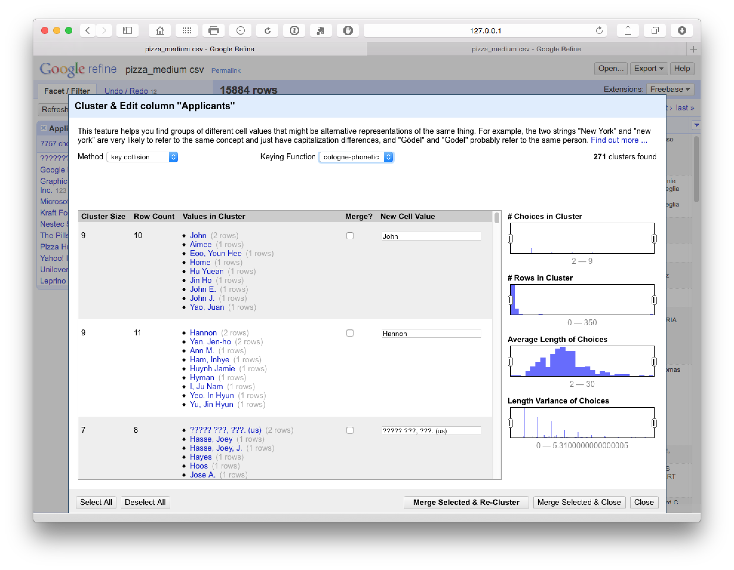
In practice, selection of items at this stage feeds into the next stage of cleaning using the Cologne-phonetic algorithm. As we can see below, this algorithm identified 271 clusters that were almost entirely clustered on the names of individuals with a limited number of accurate hits.
8.8.4 Levenshtein Edit Distance
The final steps in the process focus on Nearest Neighbour matches for our reduced number of clusters. Note that this may take some time to run (e.g. 10-15 minutes for the +7,000 clusters in this case). The results are displayed below
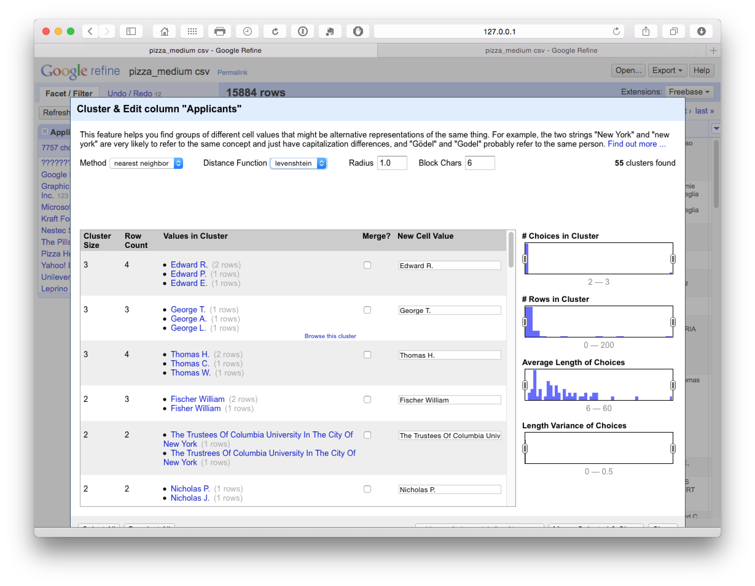
In some cases the default settings matched individual names on different initials, but in the majority of cases the clusters appeared valid and were accepted. In this case particular caution is required on the names of individuals and browsing the results to check the accuracy of matches.
8.8.5 PPM
The PPM step is the final logarithm but took so long that we decided to abandon it relative to the likely gains.
8.8.6 Preparing for export
In practice, the cleaning process will generate a new data table for export that focuses on the characteristics of applicants. To prepare for export with the cleaned group of applicant names there will be a choice on whether to retain the publication number as the single key, or, whether to use the fill down process illustrated above across the columns of the dataset. It is important to note that caution is required in the blanket use of fill down.
It is also important to bear in mind that the dataset that has been created contains many more rows than the original version. Prior to exporting we would therefore suggest two steps:
- Rerun Common transforms > to title case, to regularise any names that may have been omitted in the first round and rerun trim whitespace for any spaces arising from the splitting of names.
- Rerun facets on each column, select blank at the end of the facet panel and fill with NA. Alternatively, do this immediately following export.
8.9 Round Up
In this chapter we have covered the main features of basic data cleaning using Open Refine. As should now be clear, while it requires an investment in familiarisation it is a powerful tool for cleaning up small to medium sized patent datasets such as our 10,000 pizza patent records. However, a degree of patience, caution and forward planning is required to create an effective workflow using this tool. It is likely that further investments of time (such as the use of regular expressions in GREL) would improve cleaning tasks prior to analysis.
Open Refine is also probably the easiest to use free tool for separating and cleaning applicant and inventor names without programming knowledge. For that reason alone, while noting the caveats highlighted above, Open Refine is a very valuable tool in the open source patent analytics toolbox.
8.10 Useful Resources
The Open Refine website has links to lots of useful resources including video walkthroughs
