Introduction
The USPTO has implemented a patent visualization and analysis platform named Patentsview
Show code
knitr::include_graphics("images/patentsview/fig1_front.png")
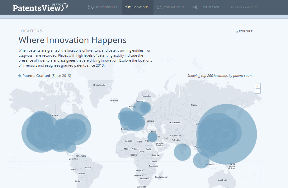
Patentsview is openly available through the web and enables the discovery and exploitation of US patent data in a visual, convenient way.
It makes it particularly easy to check out which are the most patented technologies, the main patent assignees within each technology area and the most prolific inventors. All these relationships, the associated locations and the data can be interactively explored and compared.
There is also an associated API for developers to personalise queries and download the corresponding patent data.
Moreover, an R package is available to access to Patentsview data from R. Let’s check it out.
Patentsview from R
With the patentsview package we can access, search and analyse USPTO patent data available in Patentsview.
First, we need to install and load the required packages (together with Patentsview we will also use the package highcharter allowing us to generate interactive visualizations of the data we obtain).
Show code
library(patentsview)
library(tidyverse) # for data manipulation
library(highcharter) # wrapper of highchart library to generate interactive visualisations
We can then formulate our patent queries using specified search fields.
We will need to express them using the function: with_qfuns (to list query functions to be used) and then concatenate searches in each data field we want to search with corresponding operator functions; p.e. dates with gte(patent_date = "2016-01-01 (where gte stands for greater or equal) or exact terms in textual fields (p.e. in the abstract) with text_all(patent_abstract = "UAS") or specific Cooperative Classification Classes (CPCs) using: qry_funs$eq(cpc_subsection_id = "G12").
Here is just a query formulation example considering a series of synonyms and a series of related classes:
Show code
library(patentsview)

query <-
  with_qfuns(
    and(
      gte(patent_date = "2016-01-01"),
      or(
        text_all(patent_abstract = "UAS"),
        text_all(patent_abstract = "drones"),
        text_all(patent_abstract = "UAV"),
        text_all(patent_abstract = "commercial"),
        text_all(patent_abstract = "mobility"),
        text_all(patent_abstract = "traffic"),
        text_all(patent_abstract = "urban"),
        text_all(patent_abstract = "cities"),
        text_all(patent_abstract = "public"),
        text_all(patent_abstract = "security"),
        text_all(patent_abstract = "city"),
        text_all(patent_abstract = "unmanned"),
        text_all(patent_abstract = "aerial")
    ),
      or(
        qry_funs$eq(cpc_subsection_id = "G02B"),
        qry_funs$eq(cpc_subsection_id = "G09B"),
        qry_funs$eq(cpc_subsection_id = "G01"),
        qry_funs$eq(cpc_subsection_id = "G21K"),
        qry_funs$eq(cpc_subsection_id = "B64"),
        qry_funs$eq(cpc_subsection_id = "G08"),
        qry_funs$eq(cpc_subsection_id = "G05"))
    )
  )
Some of the operators that can be used are:
- eq - Equal to
- neq - Not equal to
- gt - Greater than
- gte - Greater than or equal to
- lt - Less than
- lte - Less than or equal to
- begins - The string begins with the value string
- contains - The string contains the value string
- text_all - The text contains all the words in the value string
- text_any - The text contains any of the words in the value string
- text_phrase - The text contains the exact phrase of the value string Of course, in combination with booleans (and, or, not).
Once we are happy with our search, we need to create a list containing the fields to be used in our analysis (note that we also list location data -longitude and latitude- so we can map later on):
Show code
fields <- c("patent_number", "assignee_organization",
            "patent_num_cited_by_us_patents", "app_date", "patent_date",
            "assignee_total_num_patents", "forprior_country", "assignee_id", "assignee_longitude", "assignee_latitude")
We then send our HTTP request to the PatentsView API to get the data:
Show code
library(patentsview)
pv_out <- search_pv(query = query, fields = fields, all_pages = TRUE) # this is crapping out
Show code
save(pv_out, file = "data/pv_out.rda", compress = "xz")
Show code
load("data/pv_out.rda")
Show code
# we have to unnest the data frames that are stored in the assignee list column:
dl <- unnest_pv_data(data = pv_out$data, pk = "patent_number")
Show code
save(dl, file = "data/dl.rda", compress = "xz")
Show code
load("data/dl.rda")
Identifying top assignees
Now that we got the data, let’s try to identify top assignees.
Show code
library(tidyverse)
# We create a data frame with the top 75 assignees:
top_asgns <-
  dl$assignees %>%
  filter(!is.na(assignee_organization)) %>% # we filter out those patents that are assigned to an inventor without an organization (we want only organizations)
  mutate(ttl_pats = as.numeric(assignee_total_num_patents)) %>% #we create a numeric column (ttl_pats) with total number of patents of assignee
  group_by(assignee_organization, ttl_pats) %>% # we group assignees by total number of patents (ttl_pats)
  summarise(db_pats = n()) %>%
  mutate(frac_db_pats = round(db_pats / ttl_pats, 3)) %>% #we calculate the fraction of patents from the total patents each assignee has
  ungroup() %>%
  select(c(1, 3, 2, 4)) %>%
  arrange(desc(db_pats)) %>%
  slice(1:75)
Evolution of patent activity
We can create now a data frame with patent counts by application year for each assignee:
Show code
data <-
  top_asgns %>%
  select(-contains("pats")) %>%
  slice(1:5) %>% #we filter top 5
  inner_join(dl$assignees) %>%
  inner_join(dl$applications) %>%
  mutate(app_yr = as.numeric(substr(app_date, 1, 4))) %>% #we create a new column taking only the year form the date
  group_by(assignee_organization, app_yr) %>%
  count()
We are now ready to plot the evolution using highchartr by assigning years to de x axis and number of patents to the Y axis and grouping them by assignee organization:
Show code
library(highcharter)
data %>%
  hchart(.,
         type = "line",
         hcaes(x = data$app_yr,
               y = data$n,
                 group = data$assignee_organization)) %>%
  hc_plotOptions(series = list(marker = list(enabled = FALSE))) %>%
  hc_xAxis(title = list(text = "Published applications")) %>%
  hc_yAxis(title = list(text = "Patents on Drones")) %>%
  hc_title(text = "Top 5 assignees patenting on 'Commercial Drones'") %>%
  hc_subtitle(text = "Annual patent applications through time")
Top cited assignees
To get the top cited assignees, we write a ranking function that will be used to rank patents by their citation counts:
Show code
percent_rank2 <- function(x)
  (rank(x, ties.method = "average", na.last = "keep") - 1) / (sum(!is.na(x)) - 1)

# Create a data frame with normalized citation rates and stats from Step 2:
asng_p_dat <-
  dl$patents %>%
  mutate(patent_yr = substr(patent_date, 1, 4)) %>%
  group_by(patent_yr) %>%
  mutate(perc_cite = percent_rank2(patent_num_cited_by_us_patents)) %>%
  inner_join(dl$assignees) %>%
  group_by(assignee_organization) %>%
  summarise(mean_perc = mean(perc_cite)) %>%
  inner_join(top_asgns) %>%
  arrange(desc(ttl_pats)) %>%
  filter(!is.na(assignee_organization)) %>%
  slice(1:20) %>%
  mutate(color = "#18BC9C") %>%
  as.data.frame()
and we can now visualize it through a bubblechart scatterplot were the bubble size is relative to the number of patents, the position in the y axis is relative to the percentage of citations (highly cited organizations are positioned higher in the chart)
Show code
# Adapted from http://jkunst.com/highcharter/showcase.html
hchart(asng_p_dat, "scatter", hcaes(x = db_pats, y = mean_perc, size = frac_db_pats,
                                    group = assignee_organization, color = color)) %>%
  hc_xAxis(title = list(text = "Patents on Drones"), type = "logarithmic",
           allowDecimals = FALSE, endOnTick = TRUE) %>%
  hc_yAxis(title = list(text = "Mean percentile of citation")) %>%
  hc_subtitle(text = "Most cited assignees on 'Drones'", align = "center") %>%
  hc_add_theme(hc_theme_538()) %>%
  hc_legend(enabled = FALSE)
Origin of inventions
Using the mapping library leaflet and CartoDB data -and given that we had longitude and latitude fields- we can geomap assignee organizations around the globe. We make the bubble size relative to the applicant’s number of patents.
Show code
library(leaflet)
library(htmltools)
library(dplyr)
library(tidyr)

datad <-
  pv_out$data$patents %>%
    unnest(assignees) %>%
    select(assignee_id, assignee_organization, patent_number,
           assignee_longitude, assignee_latitude) %>%
    group_by_at(vars(-matches("pat"))) %>%
    mutate(num_pats = n()) %>%
    ungroup() %>%
    select(-patent_number) %>%
    distinct() %>%
    mutate(popup = paste0("<font color='Black'>",
                          htmlEscape(assignee_organization), "<br><br>Patents:",
                          num_pats, "</font>")) %>%
    mutate_at(vars(matches("_l")), as.numeric) %>%
    filter(!is.na(assignee_id))

pd <- leaflet(datad) %>%
  addProviderTiles(providers$CartoDB.PositronNoLabels) %>%
  addCircleMarkers(lng = ~assignee_longitude, lat = ~assignee_latitude,
                   popup = ~popup, ~sqrt(num_pats), color = "#18BC9C")
pd