Chapter 4 Counting Patent Data

This chapter provides an in depth introduction to the development of descriptive patent statistics. The most important existing resource for the development of patent statistics is the OECD Patent Statistics Manual and a series of OECD working papers (OECD Patent Statistics Manual 2009). However, a practical step by step guide to the development of patent counts using real world data has been lacking. This chapter aims to fill this gap by working up from the analysis of the structure of patent numbers through to the creation of counts of priority or first filings. We then focus on exploring patent families and conclude by graphing patent trends. Our aim is to provide a solid platform in issues involved in counting patent data that will allow you to explore more advanced techniques in the future (such as modelling and forecasting).

The Chapter makes extensive use of the drones patent dataset. The drones dataset is a set of patent documents from Clarivate Analytics Derwent Innovation database relating to the term drone or drones created as a toy or training dataset for experiments in developing patent statistics. Instructions on how to install it are provided the How to Use the Handbook section at the front of the book and on the dataset home page.

4.1 The structure of patent numbers

Patent numbers are the key identifiers for patent documents. At the time of writing there are over 107 million patent and related documents within the European Patent Office central DOCDB. The key to working with and counting these documents is an understanding of the structure of patent numbers.

Table 4.1 presents the main patent numbers as they are commonly retrieved from patent databases.

Table 4.1: Examples of Types of Patent Numbers

row	priority_number	application_number	publication_number
1	US2016578323F 2016-09-20	US2016578323F 2016-09-20	USD801224S1
2	US15360203A 2016-11-23	US15360203A 2016-11-23	US9807726B1
3	US62133061P 2015-03-13	US15069675A 2016-03-14	US9804596B1
4	US14622134A 2015-02-13	US14622134A 2015-02-13	US9802728B1
5	JP2015122335A 2015-06-17; WO2016JP67809A 2016-06-15	US15322008A 2016-12-23	US9802691B2
6	US15346251A 2016-11-08	US15346251A 2016-11-08	US9805273B1

For each of these numbers we observe the following structure

1. A two letter country code such as US (United States) or KR (South Korea)
2. A numeric identifier that, for more recent years, may include the year e.g 2016578323 or 15263985
3. A letter or combination of a letter and a number such as A, A1, B1, B2, S or P denoting what is called the Kind code for the document
4. The date in Year - Month - Day format (known as YYYY-MM-DD)

It is important to note that the patent numbers retrieved from patent databases are not necessarily presented in the way they are stored. For example, the country code, the numeric identifier, the kind code and the date are often stored in separate columns and are then combined together. When working with different databases this can be reflected in spaces or underscores between the country code, the number and the kind code. In addition, the original entries on patent application forms often include forward slashes /. In some cases databases will present numbers containing the forward slash character and in others they will be deleted as they do not add to the distinctiveness of the identifier. Be aware that some patent databases, notable Derwent Innovation from Clarivate Analytics, add padding 000s in the middle of some patent numbers to make them uniform and may add the year field at the beginning of patent numbers. For this reason using patent numbers across different databases is not as straightforward as it might be. Slight variations in the format will be the most common reason that a patent number is found in one database but not in another.

4.1.1 The country code

The two letter country code denotes either the country of filing, the country of application or the publication country. For example, in row 5 of Table 4.1 above, JP2015122335A 2015-06-17 was first filed as an application in Japan (JP) and then went forward to the Patent Cooperation Treaty as WO2016JP67809A 2016-06-15 (where WO denotes the Patent Cooperation Treaty). That application was then submitted as US15322008A 2016-12-23 in the United States (US) and published as US9802691B2. A full list of two letter country codes, including the codes for the Patent Cooperation Treaty (WO) and regional instruments is available in the WIPO Handbook on Industrial Property Information and Documentation under standard ST.3 Recommended Standard on two-letter Codes for the Representation of States, Other Entities and Intergovernmental Organizations. The same table is also available on Wikipedia. Software tools such as VantagePoint provide thesauri that will convert country codes to country names. Software packages such as countrycode in R are designed to facilitate data science work and often include various formats for country code systems that you might encounter as well as providing country names in relevant languages.

The country codes tell us where a document is filed and published. This provides the foundation for identifying trends by country using a range of different counts and for geographic mapping.

4.1.2 The numeric identifier

The second element of a patent number is a numeric identifier. As noted above, it is important to note that these identifiers may be edited by databases. For example, the Derwent World Patent Index often uses either a single or padding zero between the year in a field and the number. This probably arose from an effort to make patent numbers a uniform length but has the effect that these documents cannot easily be retrieved from databases that do not use padding zeros (such as esp@cenet). In other cases the numbers may include characters such as “/” that are not formally speaking part of the identifier. The kind code may also be added in some databases but not in others.

4.1.3 Kind Codes

Kind Codes appear as letter and number combinations after the numeric identifier. Kind codes describe the type of document and its publication level. Kind codes are documented in WIPO Standard ST.16 Recommended Standard Code for the Identification of Different Kinds of Patent Documents. Formally speaking Kind Codes are applied to:

“patents for invention, inventors’ certificates, medicament patents, plant patents, design patents, utility certificates, utility models, patents or certificates of addition, utility certificates of addition, and published applications therefor” (WIPO ST.16 page 3.16.1, October 2016)

In connection with the publication level, the definition explains that:

“a “publication level” is defined as the level corresponding to a procedural stage at which normally a document is published under a given national industrial property law or under a regional or international industrial property convention or treaty.”

So, to take a common example, a patent document may be published at the application stage. This is commonly the first procedural stage and is the first publication level. In many countries, standard patent applications will receive the kind code A at this first publication level. In many cases, when a patent is granted the document enters the second publication level and it is published with kind code B. Other types of patent documents commonly receive their own kind codes denoting their type. For example Utility Models receive the kind code U while design patents received kind code S.

Kind codes are often accompanied by a number that adds additional information about the type of document. Within the WIPO standard these numbers range from 1 to 7 with numbers 8 and 9 reserved for corrections to the bibliographic data (e.g. A8) or to any part of the document (e.g. A9). WIPO Examples and Kinds of Patent Documents forms part of the WIPO Handbook on Industrial Property Information and Documentation setting out common Kind Codes and is recommended reading for patent analysts. Quick reference tables are also produced by Clarivate Analytics and national patent offices and are available online.

The use of patent kind codes has evolved over time and this can make accurate interpretation of a kind code difficult. In practice:

1. The use of a kind code may vary in the same country over time. For example in the United States prior to 2001 patents were only published when they were granted (first publication level) and they were awarded kind code A. From 2001 onwards the United States adopted common practice elsewhere and published applications which now receive kind code A (as the first publication level) while patent grants are now the second publication level (and receive kind code B);
2. The use of kind codes varies between countries.

As a very rough rule of thumb, publications with kind code A commonly mean the publication of an application. Publications with kind code B mean publication of a patent grant. But, this is not always true and it can only be described as a rough rule of thumb. This rule can normally be used when working with data from the main jurisdictions such as the United States (bearing in mind the pre and post 2001 changes considered below), the European Patent Office and the Patent Cooperation Treaty (which only covers first level publications or applications) and Japan. However, when working with country level data to elaborate trends for applications and grants it is important to review the use of kind codes in each country to be covered and to identify changes in the use of kind codes over time. When developing data on statistical trends for applications and grants a note should normally be added to inform readers that the data is approximate in cases where the use of kind codes has not been thoroughly explored and documented.

Patent kind codes denoting publication level and the kind of document (e.g. U) are important for statistical purposes because they allow for the identification of duplicates and, depending on the purpose of the analysis, the removal of unwanted data types (such as Utility models, design patents and plant patents) or the isolation of specific types of document. For most purposes kind codes are important for identifying patent applications and grants and critically for identifying republications of the same document (duplicates)

The most common kind codes encountered in patent data are:

First publication level (commonly but not exclusively patent applications)

• A1
• A2
• A3

Second publication level (commonly but not exclusively patent grants)

• B1
• B2
• B3

This means, to take a fictional example from the USPTO and its common kind codes reference table, that:

• US1234A1 Patent Application Publication
• US1234A2 Patent Application Publication (Republication)
• US1234A9 Patent Application Publication (Corrected Publication)
• US1234B1 Granted Patent (not previously published as a patent application)
• US1234B2 Granted Patent (previously published as a patent application)

In this example we have 3 potential publications of the same application and one publication of a patent grant (although corrections to a granted patent are possible). For the purpose of counting patent data how we deal with these republications or duplicates depends on the question we are trying to answer.

If we wanted to identify the priority application that is closest to the investment in research and development we would choose the earliest application number available to us (that may or may not have been published). In other cases we may want to count all applications that stem from a first filing or set of filings while in others we may want to identify applications and grants but remove administrative republications (simple republications and corrections or publication of the international search report) from the counts.

The main issue that arises here is determining what we wish to include and exclude from counts. One general approach to this issue is to simply remove all republications of the same document (count the document only once on the earliest in the series) . For example, if we were interested in counting patent applications and patent grants in the United States we would count US1234A1 and we would count the patent grant (US1234B2) and exclude the republications of the application. If we are only interested in counting patent applications we might simply remove the kind code denoting the different publication levels to count document US1234 only once. In practice, basic patent statistics commonly involves the use of multiple counting methods as we will see in more detail below.

As the discussion above makes clear when working with patent data to elaborate patent counts we must address multiplier effects. These take two main forms:

1. Republication of the same basic document in the same jurisdiction as applications, grants, or with modifications as continuations, continuations in part, divisionals or corrections.
2. Submission of applications under regional patent instruments or the Patent Cooperation Treaty (WO) and their republication as applications, grants, other administrative publications or divisionals (in relevant jurisdictions).

Thus, under the Patent Cooperation Treaty an applicant may submit the same patent application for consideration in up to 156 Contracting States. In practice this is rare but in theory a single application could potentially lead to the republication of the same document as an application and grant up to 312 times (assuming a single publication of an application and the publication of a grant in each country). While this would be a very unusual case, it reveals the potential multiplier effects in patent counts introduced by regional instruments such as the European Patent Convention and the Patent Cooperation Treaty. As we will see below, in some cases a single document may be linked to over 1000 publications.

4.2 Preparing to Count Patent Data

The patent identifiers discussed above provide the key for tracking patent documents around the world, using the concept of patent families discussed below, and for elaborating patent counts. The most important single piece of information when thinking about patent counts using identifiers is that patent patent data involves multiplier effects that often leads to the duplication or republication of the same document or a document that has been modified based on an earlier version. Patent identifiers provide the basis for navigating these multiplier effects. The basis for patent counts commonly consists of removing duplicates or deduplication at different levels or combining documents in a variety of ways.

We will use the drones dataset as an example of this. Table 4.2 shows a sample of different patent numbers.

Table 4.2: Priority, Applications, Publication and INPADOC Family Members

row	priority_number	application_number	publication_number	inpadoc_family_members
9	US2016620248F 2016-09-02	US2016620248F 2016-09-02	USD800603S1	USD800603S1 20171024
10	US14835329A 2015-08-25	US14835329A 2015-08-25	US9801234B2	US20170064599A1 20170302; US9801234B2 20171024
11	US15174819A 2016-06-06	US15174819A 2016-06-06	US9800796B1	US9800796B1 20171024
12	US14530548A 2014-10-31; US2013898275P 2013-10-31	US14530548A 2014-10-31	US9800517B1	US9800517B1 20171024
13	US2015274112P 2015-12-31; US2016341797A 2016-11-02; US2016341809A 2016-11-02; US2016341813A 2016-11-02; US2016341818A 2016-11-02; US2016341824A 2016-11-02; US2016341831A 2016-11-02; US62274112P 2015-12-31	US15341809A 2016-11-02	US9800321B2	CN106878672A 20170620; CN106982345A 20170725; CN107040754A 20170811; CN107046710A 20170815; CN107070531A 20170818; CN107071794A 20170818; CN206481394U 20170908; CN206517444U 20170922; EP3188474A1 20170705; EP3188475A1 20170705; EP3188476A1 20170705; EP3188477A1 20170705; EP3190788A1 20170712; EP3190789A1 20170712; US20170193556A1 20170706; US20170193820A1 20170706; US20170195038A1 20170706; US20170195048A1 20170706; US20170195627A1 20170706; US20170195694A1 20170706; US9786165B2 20171010; US9800321B2 20171024; WO2017114496A1 20170706; WO2017114501A1 20170706; WO2017114503A1 20170706; WO2017114504A1 20170706; WO2017114505A1 20170706; WO2017114506A1 20170706

We can see here that one or more priority numbers are linked to application numbers. In some cases those numbers are identical while in other cases they are distinct. The application number is linked to one or more publication numbers. Patent databases commonly return data based on publication numbers. However, this is often only a partial picture of the set of documents linked to an application or set of applications and their underlying priority filings.

In the rows 10 and 13 in Table 4.2 we can see that we have one publication number. However, we can see that under the INPADOC Family Member Number there are multiple patent publications that are not captured in the publication number field. There are two reasons for this.

1. A search of a patent database commonly returns patent publications based on criteria such as limiting the search by jurisdiction. This does not reveal all documents linked to a filing or set of filings worldwide.
2. The INPADOC Family Members column groups publications based on a particular definition of a patent family. The number of documents will vary here depending on the definition of the patent family used in the data and whether the documents are deduplicated.

Table 4.3 summarises the data by showing the counts of the different types of documents.

Table 4.3: Sample of Patent Counts linked to the earliest priority number

earliest_priority	priority_count	application_count	family_count
US2016620248F 2016-09-02	1	1	1
US14835329A 2015-08-25	1	1	2
US15174819A 2016-06-06	1	1	1
US2013898275P 2013-10-31	2	1	1
US2015274112P 2015-12-31	8	18	28
US201476360P 2014-11-06	7	4	7

Table 4.3 helps to make clear that we may be dealing with simple cases (one priority or first filing) leads to one application and one family member. Or, we may be dealing with a group of priorities leading to multiple applications and multiple family members. This helps to clarify that, when working with patent data we are often dealing with many to many relationships.

In the next section we will progressively move up from counting patent documents using priority numbers and finish by using counts of INPADOC family members to elucidate trends for drone related technology.

4.3 Understanding Priority Numbers

When a patent application is filed for the first time anywhere in the world it becomes the priority document or first filing. The use of this term is based on the 1883 Paris Convention. The WIPO summary of the key provisions of the Paris Convention explains the right of priority introduced by the Convention as follows.

The Convention provides for the right of priority in the case of patents (and utility models where they exist), marks and industrial designs. This right means that, on the basis of a regular first application filed in one of the Contracting States, the applicant may, within a certain period of time (12 months for patents and utility models; 6 months for industrial designs and marks), apply for protection in any of the other Contracting States. These subsequent applications will be regarded as if they had been filed on the same day as the first application. In other words, they will have priority (hence the expression “right of priority”) over applications filed by others during the said period of time for the same invention, utility model, mark or industrial design. Moreover, these subsequent applications, being based on the first application, will not be affected by any event that takes place in the interval, such as the publication of an invention or the sale of articles bearing a mark or incorporating an industrial design. One of the great practical advantages of this provision is that applicants seeking protection in several countries are not required to present all of their applications at the same time but have 6 or 12 months to decide in which countries they wish to seek protection, and to organize with due care the steps necessary for securing protection.⁸

The OECD Patent Statistics Manual describes the priority number and the priority date as follows:

Priority number. This is the application or publication number of the priority application, if applicable. It makes it possible to identify the priority country, reconstruct patent families, etc.

Priority date. This is the first date of filing of a patent application, anywhere in the world (usually in the applicant’s domestic patent office), to protect an invention. It is the closest to the date of invention. (OECD 2009: 25)

The most important issue here from the perspective of patent counts is the priority date. Table 4.3 above revealed that patent applications may be linked to multiple underlying priority applications. The earliest filing, as shown in Table 4.3, is the Paris priority in the sense that it is the first of a set of filings giving rise to a claimed invention.

In the simple cases shown in rows 9-11 of Table 4.2, the priority number and the application number are the same. Where the priority number and the application number are the same, we have identified the priority or first filing. However, in rows 12-13 in Table 4.2 we see more complex cases involving multiple priorities. In row 5 of Table 4.4 we see a common case where a national level filing gives rise to an international filing under the Patent Cooperation Treaty that leads to an application in another country. In the remainder of this section we will walk through a number of examples.

1. National Filing to International Filing

First let’s look at the example in row 5 of Table 4.2.

Table 4.4: Priority, Applications, Publication and INPADOC Family Members

priority_number	application_number	publication_number	inpadoc_family_members
US2016578323F 2016-09-20	US2016578323F 2016-09-20	USD801224S1	NA
US15360203A 2016-11-23	US15360203A 2016-11-23	US9807726B1	NA
US62133061P 2015-03-13	US15069675A 2016-03-14	US9804596B1	NA
US14622134A 2015-02-13	US14622134A 2015-02-13	US9802728B1	NA
JP2015122335A 2015-06-17; WO2016JP67809A 2016-06-15	US15322008A 2016-12-23	US9802691B2	NA

We can see in row 5 that JP2015122335A 2015-06-17 lists a second priority number for a Patent Cooperation Treaty filing WO2016JP67809A 2016-06-15. At first sight this leads to US patent application US15322008A 2016-12-23 that is published as US9802691B2 for a Buoyant Aerial Vehicle. However, when working with priority numbers we commonly encounter multiple applications arising from the priorities. Table 4.5 displays counts of the priorities and applications linked to JP2015122335A 2015-06-17.

Table 4.5: Applications arising from JP2015122335A 2015-06-17

earliest_priority	priority_count	application_count
JP2015122335A 2015-06-17	2	4

The second priority number is the Patent Cooperation Treaty WO2016JP67809A 2016-06-15.

Table 4.6 shows the sequence of applications arising from the two priorities and the INPADOC patent family.

Table 4.6: Patent Applications arising from JP2015122335A with PCT application WO2016JP67809A

priority_number	application_number	publication_number	inpadoc_family_members
JP2015122335A 2015-06-17	US15322008A 2016-12-23	US9802691B2	NA
JP2015122335A 2015-06-17	EP2016811654A 2016-06-15	EP3150483A1	EP3150483A1 20170405; EP3150483A4 20170920; JP05875093B1 20160302; JP2017007411A 20170112; US20170137104A1 20170518; WO2016204180A1 20161222
JP2015122335A 2015-06-17	WO2016JP67809A 2016-06-15	WO2016204180A1	EP3150483A1 20170405; EP3150483A4 20170920; JP05875093B1 20160302; JP2017007411A 20170112; US20170137104A1 20170518; WO2016204180A1 20161222
JP2015122335A 2015-06-17	JP2015122335A 2015-06-17	JP05875093B1	EP3150483A1 20170405; EP3150483A4 20170920; JP05875093B1 20160302; JP2017007411A 20170112; US20170137104A1 20170518; WO2016204180A1 20161222

The first point to note is that Japanese priority application JP2015122335A 2015-06-17 becomes application JP2015122335A 2015-06-17 and is then published as a patent application in Japan as JP2017007411A 20170112 in January 2017 (first publication level) and also as a granted patent JP05875093B1 20160302.⁹

However, the Patent Cooperation Treaty application WO2016JP67809A 2016-06-15 filed a year later triggers applications (on the same date) in the United States and at the European Patent Office.

Application number US15322008A 2016-12-23 is published in May 2017 as US20170137104A1 20170518 (first publication level) and on the second publication level as US9802691B2.

European application EP2016811654A 2016-06-15 is published as EP3150483A1 20170405 (first publication level with the search report) and as EP3150483A4 20170920 with a supplementary search report.

Note here that the database entry for the INPADOC family members for the United States application is blank (NA stands for Not Available) indicating that this record had not been updated or correctly updated. An up to date view of the patent family is available from esp@cenet and includes the US records and more recent patent activity.

The priority data in this case reflects the decision taken by the applicant on the filing route to pursue protection in other countries in this case the United States using the Patent Cooperation Treaty. The Patent Cooperation Treaty has the advantage of extending the time that applicants enjoy before deciding where else to pursue protection from 12 months under the Paris Convention to up to 30 months. Applicants also enjoy reduced costs compared with the Paris Convention because a single application is submitted that may then go forward for consideration in other Contracting States.

Note that the filing route can be detected in the priority number WO2016JP67809A 2016-06-15 which contains the country code JP as part of the application number. It is commonly the case that the listing of priorities numbers follows a sequence where the first priority number listed on a document is the earliest, followed by later applications. This common pattern may give rise to the temptation to simply take the first priority number in a sequence of priorities as the earliest priority. However, experience demonstrates that databases are not consistent in listing the earliest filing in this way. The temptation should therefore be resisted.

As this example makes clear when working with patent data we are typically following a pattern consisting of:

priority number (earliest) > application number > publications (under different family definitions)

At each step the publications associated with the original filings multiply.

In this case we are observing the distinctive filing route arising from a single priority filing. The filing route has nothing to do with the invention per se. However a more complex example reveals that inventions may arise from multiple claimed inventions.

2. Multiple Inventions

We have seen above that in some cases patent applications involve multiple priority numbers. Most will follow the pattern identified above. However, in some technology areas, notably those involving computing, multiple priority numbers may be quite common. In the case of the drones dataset a single application US14815121A 2015-07-31 lists no less that 146 priorities and has given rise, at the time of writing, to an INPADOC patent family consisting of 340 publications. This example concerns a Wireless Power System for an Electronic Display with Associated Impedence Matching Network. It can be identified in esp@cenet using publication number US2015357831A1 and a summary is presented in Table 4.7.

Table 4.7: Multiple Priorities and US Provisional and Continuation Filings

priority_country	n
AU	1
TW	1
US	144

Table 4.7 reveals that the majority of priorities are domestic US priorities (144) with two foreign priorities in the form of Australia and Taiwan.

The earliest priority filing listed in the set of priorities is US2007647705A 2007-12-28 and the latest are in 2017 signifying that the underlying filings linked to this application spanned nearly a decade. Of the 143 priorities linked to the application originating from the United States 107 carry kind code A and 36 contain kind code P for a Provisional application. This therefore appears to be a case dominated by US provisional and so called continuation, continuation in part and divisional applications.

Provisional applications are a common type of patent application in the United States where an applicant may submit and claim priority to what is effectively an outline of a full application that does not contain patent claims. These applications serve to establish an early priority date but this does not take effect until an actual application is filed. Provisional applications are not published. Details of the procedures for these types of patent applications are found in the USPTO Manual of Patent Examining Procedure (MPEP).

In the United States applicants are also allowed to file continuation and continuation in part applications. In the case of continuations the applicant adds new claims that claim priority to the earlier filed application. In the case of continuation in part, these applications add new subject matter focusing on enhancements to the original application. Divisional applications claim priority to the original application but claim distinct new inventions rather than adding new claims or subject matter. Divisional applications often arise where the examiner determines that an application contains more than one invention.

The use of continuation and continuation in part applications in the United States has been a significant focus of debate and criticism (Hegde, Mowery, and Graham 2007). As Dechezlepretre et. al. have recently highlighted:

“At the national or regional levels, applicants can in turn use second domestic filings, including divisional and continuing applications, to delay a patent grant. By filing a divisional application while the parent application is still pending, applicants can obtain a second (or possibly more) divisional patent(s) granted later, and meanwhile maintain some uncertainty on the claims. In the U.S. patent system, continuations and continuations-in- part can be filed after the examination, and aim precisely at adding more claims to a patent (Hegde et al. 2009). Filing a first application with narrow claims thus makes it possible for the applicant to obtain several patents on the same invention, thereby gradually extending the overall scope of the claims and even, in the case of continuations-in-part, the duration of the patent family.” (Dechezleprêtre, Ménière, and Mohnen 2017 at 802)

While the cases where have discussed above are straightforward where this is one priority number, when focusing on US continuation filings the question that arises here is what should be counted?

Having gained an understanding of some of the potential issues involved in preparing to count patent data we now turn to methods for counting priority applications

4.4 Counting Priority Applications

Counts of priority filings are widely used in patent statistics and economic analysis because they focus attention on the relationship between the filing of an application for an invention and the underlying investment in Research and Development leading to the invention. Viewed from this perspective, and as highlighted in the OECD Patent Statistics Manual, the earliest filing of a patent application provides a proxy indicator for investments in Research and Development in a particular technology area. This information can therefore be used as a basis for identifying and exploring trends.

Within the economics literature the preference therefore is for identifying and counting the earliest priority filing in a set of priorities. This is the approach that we will adopt here. However, the discussion of the Witricity case above involving multiple filings also reveals that we should be aware of some of the potential limitations of that approach. Thus, as mentioned above the priority filing of a patent application normally corresponds with the identical application number in the priority field. However, in the Witricity case the earliest filing was listed in December 2007 while the application was in mid-2015 roughly 7 years after the original filing. This raises the question of whether the date corresponding with the specific claimed invention should be taken or whether the earliest date should be taken as the basis for the proxy indicator.

In practice, in purely methodological terms, it is easiest to identify the earliest priority in a set as the basis for elucidating trends in priority filings. However, this type of issue helps to illustrate that counts of priority filings are a proxy for underlying investments in Research and Development or in formal terms an output indicator and depending on your needs may merit refinement to more closely match the required granularity.

Counting patent filings by priority involves 8 basic steps

1. Checking the priority field for missing priority data (we can’t count missing data);
2. Separating out the concatenated column containing priority numbers. These numbers are commonly separated with a semi-colon;
3. Removing extra white space that is revealed by the separation process;
4. Separating out the priority number and the priority date (commonly using the space between these fields);
5. Grouping the priority numbers by the application number and rank them from 1 to n with 1 being the earliest;
6. Filter the priority numbers to the earliest (rank 1);
7. Detect duplicate priority numbers arising from those that share application numbers in the source set and remove them;
8. Graph the results.

The methodological steps required for this task can be performed using tools such as Open Refine which can easily separate out the data or in VantagePoint. The key challenge is in grouping and ranking the priority numbers by the earliest data. This is most easily achieved using a programming language (such as an SQL GROUP BY, PARTITION BY and RANK) or in a language such as Python or R. In the case of R this can be achieved in the following lines of code. The code is commented to show the steps identified above.

earliest_priority <- numbers %>%
  select(priority_number, application_number) %>% 
  drop_na(priority_number) %>% # drop empty priority fields
  separate_rows(priority_number, sep = ";") %>% # separate priority numbers on ";"
  mutate(priority_number = str_trim(priority_number, side = "both")) %>% # trim white space
  separate(priority_number, into = c("priority", "priority_date"), sep = " ", remove = FALSE) %>% # extract the date 
  mutate(priority_date = lubridate::ymd(priority_date)) %>% 
  mutate(year = lubridate::year(priority_date)) %>% # add the priority year field
  mutate(priority_number = str_trim(priority_number, side = "both")) %>% # trim white space
  mutate(priority_country = str_sub(.$priority_number, 1,2)) %>% # extract the priority country
  group_by(application_number) %>%  # group by application number
  mutate(filing_order = rank(priority_date, ties.method = "first")) %>% # rank application numbers by priority date 
  ungroup() %>% # remove grouping for later calculations
  filter(filing_order == 1) %>% # filter to the earliest priority at rank 1
  mutate(duplicate_priority = duplicated(.$priority_number)) %>% # identify duplicate priority numbers
  filter(duplicate_priority == "FALSE") %>% # remove duplicate priority numbers
  select(-priority) # drop unnecessary field

While the above may appear initially appear complex it follows step 1 to 7 above. Because the data lacks a priority country and year field it extracts these fields from the data to use in graphing as the next step. The key steps in arriving at accurate counts in the above process is trimming the separated fields to remove any leading and trailing white space. Note that the amount of cleaning required is likely to vary when working with data from different databases.

The steps above reduce the dataset from 15,776 applications containing 23,382 priority numbers (after the exclusion of Not Available results) to 9,358 earliest priority numbers.

We are now in a position to graph the data. For convenience we will continue to use R and the popular ggplot2 package. The results of a raw count are presented in Figure 4.1

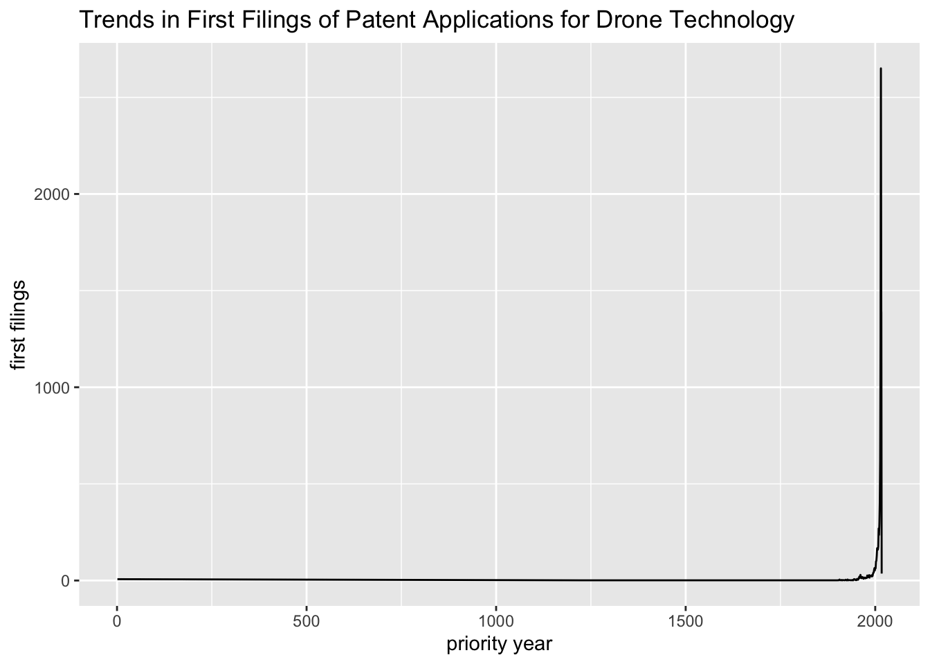
Figure 4.1: Raw Graph of Trends in Priority Filings

This is not generally what we will be expecting because it transpires that we have a long tail of low frequency records where the priority year is invalid such as 0001-01-01, or the date was not in the expected YYYY-MM-DD format. In addition this test dataset includes historic records from the 19th Century that we will not in this case be interested in seeing. It is therefore sensible to filter the results to a more recent period. Figure 4.2 shows the effect of filtering the priority year to 1990 to 2017.

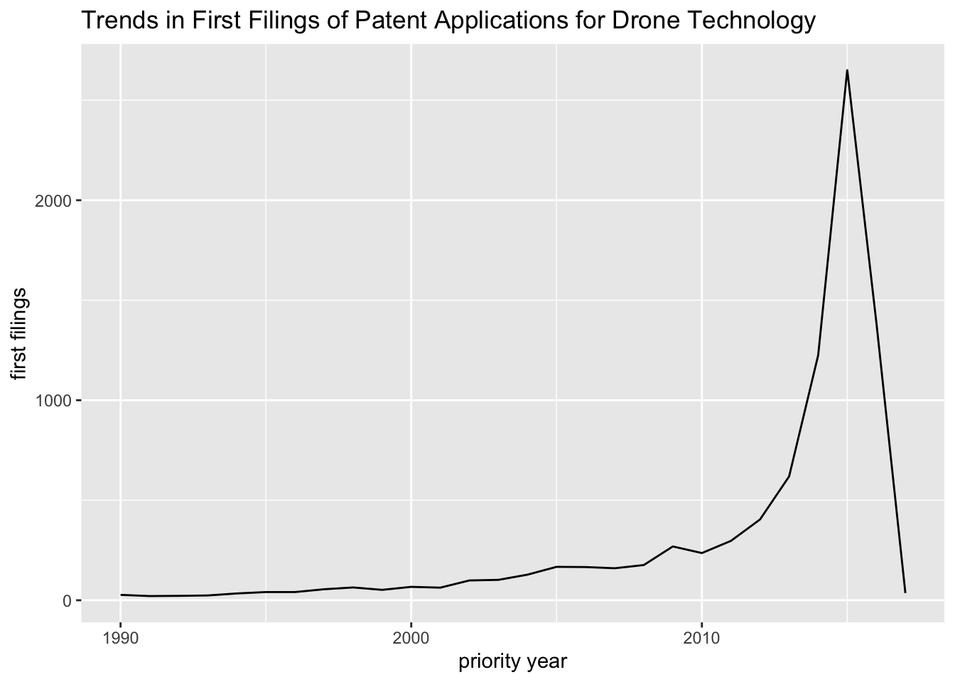
Figure 4.2: Graph of Trends in Priority Filings showing the Priority Data Cliff

This version of the graph brings us closer but note that the data falls off a cliff between 2015 and 2017. This is a characteristic of counts of patents by priority filings and you should always expect to see it. The reason it occurs is not because of a collapse in patent activity but because of the lag time between the filing of applications and their availability as publications in patent databases. The gap between the filing of an application and its publication is generally 18 months but it may be at least two years. This problem is referred to as timeliness in patent statistics. The safest option is to pull back to the date range between 2 - 3 years to avoid giving the impression of a collapse in activity. Figure 4.3 shows the effect of this approach. When using this measure it is good practice to always add a note in the account to explain why this action is taken. Equally if choosing to present the data with the data cliff present it is good practice to explain that the data cliff arises from a lack of recent data and does not reflect a change in trends in activity.

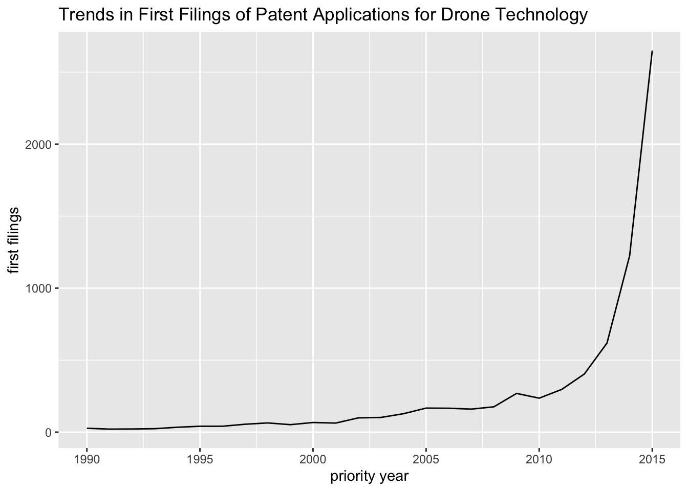
Figure 4.3: Graph of Trends in Priority Filings excluding the Data Cliff

More advanced techniques for addressing the problem of timeliness were developed by Helene Dernis at the OECD and subsequently taken forward by Eurostat (Dernis 2007, de_Rassenfosse_2013).

The key advantage of counts of the earliest priority filings is that they remove the duplication that is inherent in patent data and allows us to focus in on the underlying filing rate: that is to examine trends in filings using the dates that are closest to the underlying investment in Research and Development.

However, trends in the first filings of patent applications are not the whole story. Other types of patent counts focusing on applications, patent families and patent family members focus on the nature and geography of demand for patent rights. This will allow us to compare the implications of different types of counts.

4.5 Counting Applications

One challenge for the patent analyst is that data on priority applications may not be readily available or accessible when preparing a report. Patent databases vary in the quality of priority data and in these circumstances the use of simple counts of patent applications, accompanied by an explanatory note are likely to be an appropriate alternative. Here we need to bear in mind:

1. That we need to use the application year;
2. That we will be counting distinct applications that may arise from the same underlying filing.

Figure 4.4 shows trends in patent applications by application year.

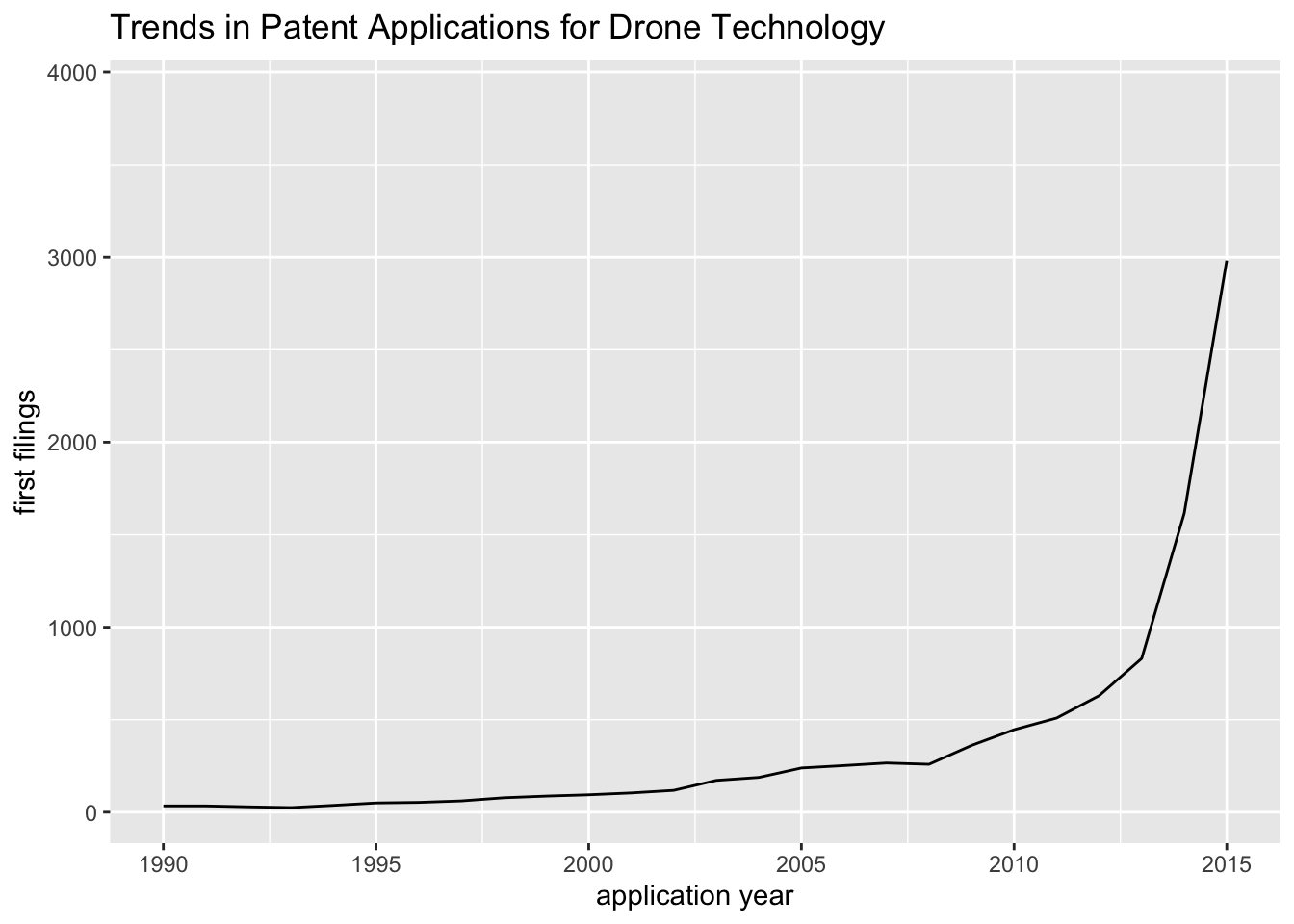
Figure 4.4: Graph of Trends in Applications by Application Year

In this case the data cliff (not shown) occurs from 2016 onwards. This reflects the fact that when compared with counts by the earliest priority year, counts by application year lean forward. Because these counts also capture the applications stemming from a priority, such as applications in more than one country, they will also be at a higher level.

Figure 4.5 compares the two figures. Figure 4.6 zooms in to the figure for the period 2005 to 2015.

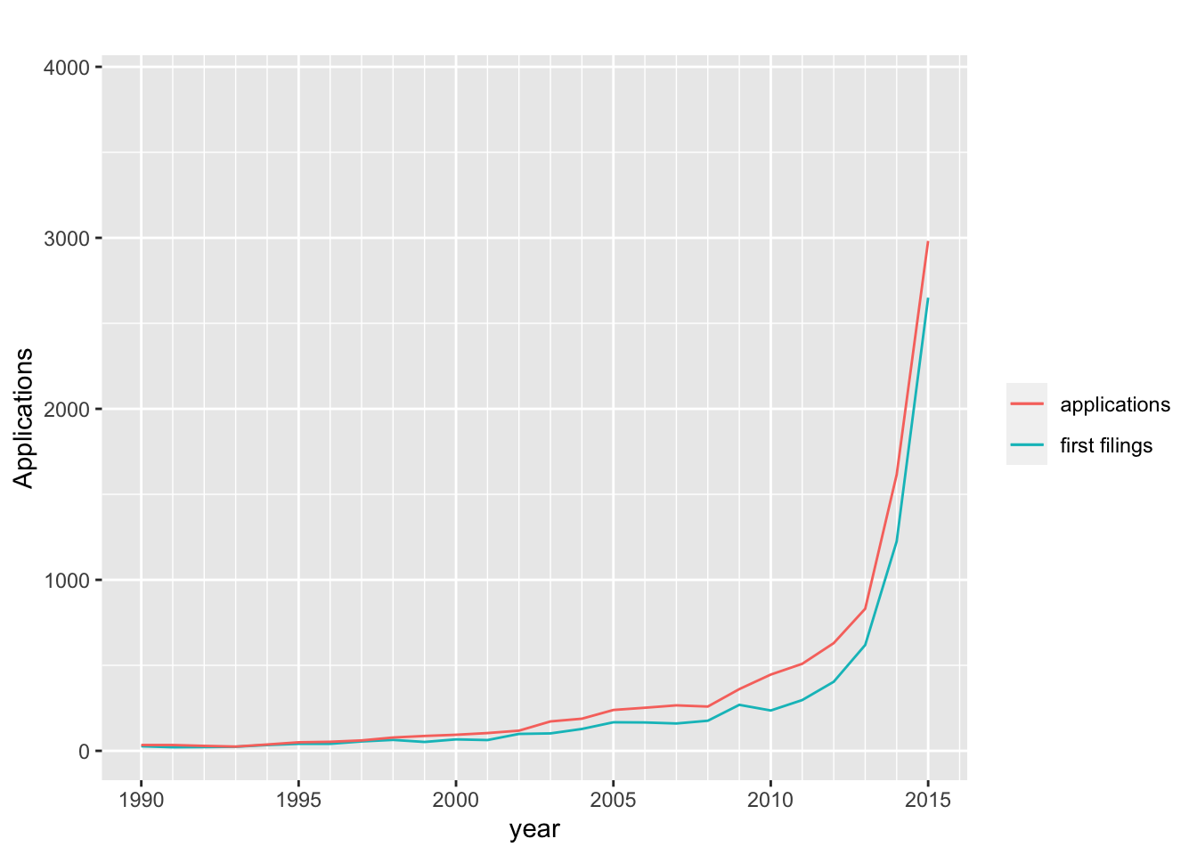
Figure 4.5: Trends in First Filings and Patent Applications

Figure 4.6 focuses in on the period 2007 to 2015 to more clearly see the divergences between the data.

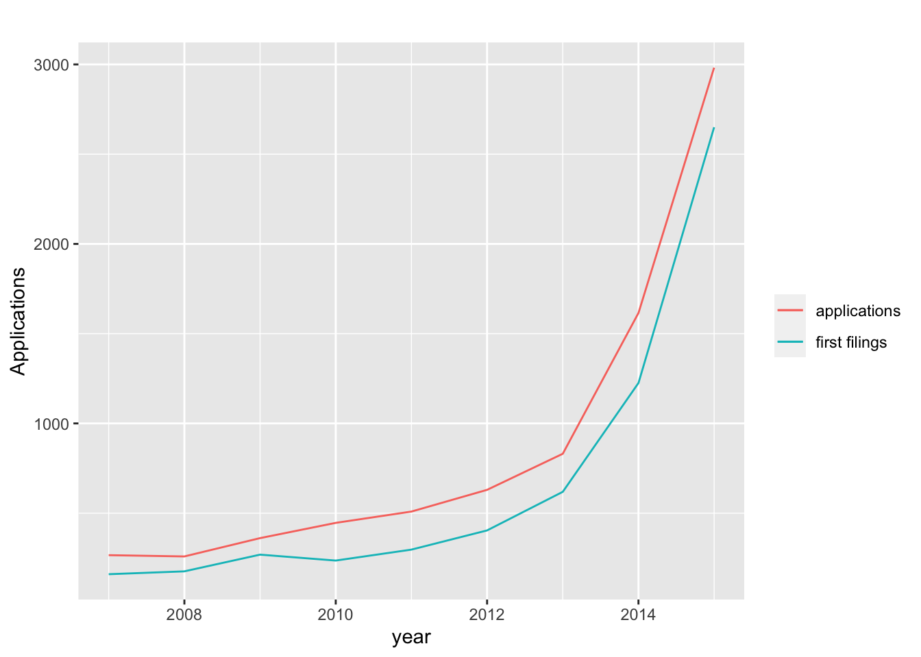
Figure 4.6: Trends in First Filings and Patent Applications

As we might expect Figure 4.5 makes clear that counts of applications run parallel to trends in first filings. However, this is not the entire picture. Note the speed bump that appears between 2007 and 2010 starting with a downward inflection in 2008 followed by an upward inflection and downward inflection in 2010 reflecting a decrease then rapid increase and decrease in first filings. While the initial downward inflexible is displayed in the trend for applications the speed bump is replaced by a steadily increasing slope until 2013.

What this reflects is the follow on multiplier effect of applications based on the underlying filings being published in multiple jurisdictions that disguises the temporary bottoming out of first filings over the same period before growth in filings accelerates dramatically.

We can also see that in 2013 an inflexible occurs in filings and applications with the inflection occurring at a higher document count for applications.

In summary, the application rate runs broadly in parallel with the priority rate but it smooths out and disguises changes in the priority filing rate that are likely to more closely reflect underlying investments in research and development.

4.5.1 Mapping Publications (Family Members)

So far we have focused on mapping trends using the earliest priority documents and application numbers. We will now examine what happens if we map patent publications using the data contained in the INPADOC family member field consisting of 49,508 publications linked to the applications and their priorities. Figure 4.7 shows the trend for counts of publications in the INPADOC family members field.

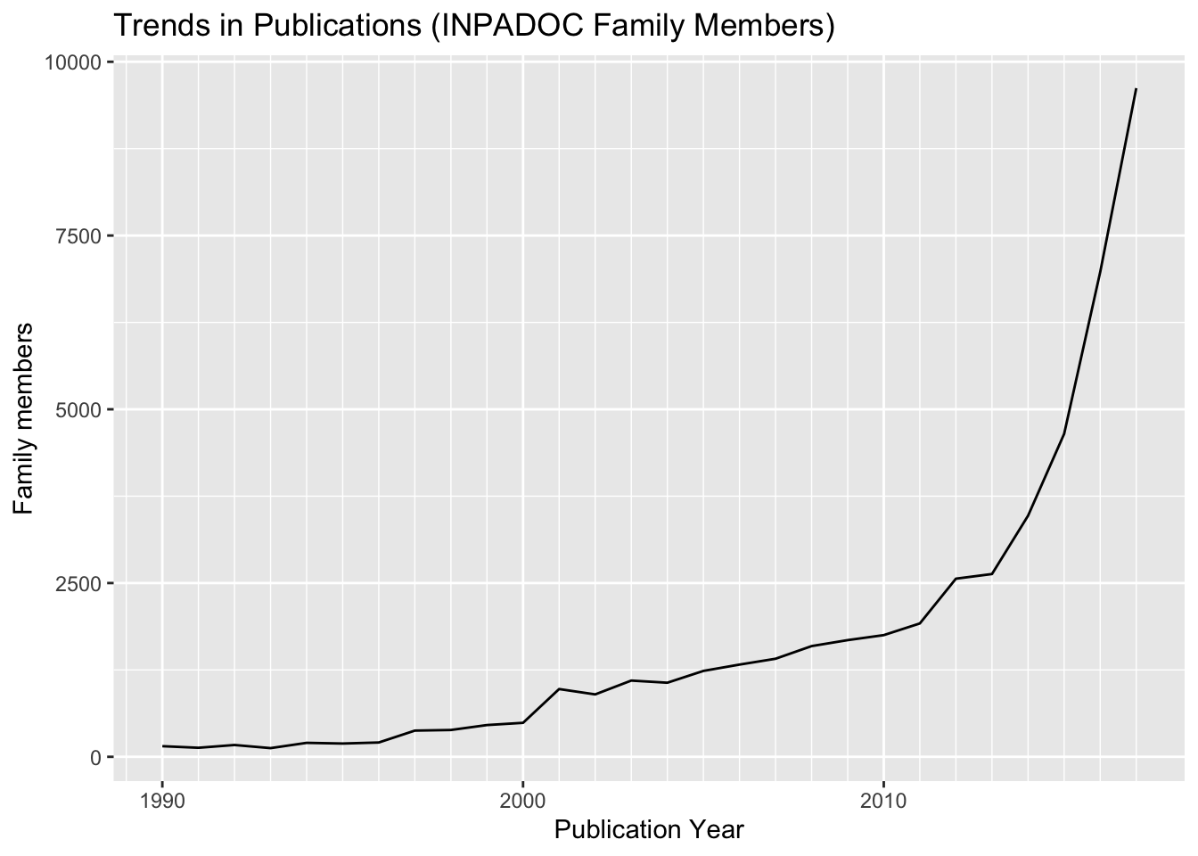
Figure 4.7: Trends in Publications (INPADOC Family Members)

We can now place this data which simply counts the number of publications within the INPADOC family members field into a graph with the counts by priority and applications as in Figure 4.8.

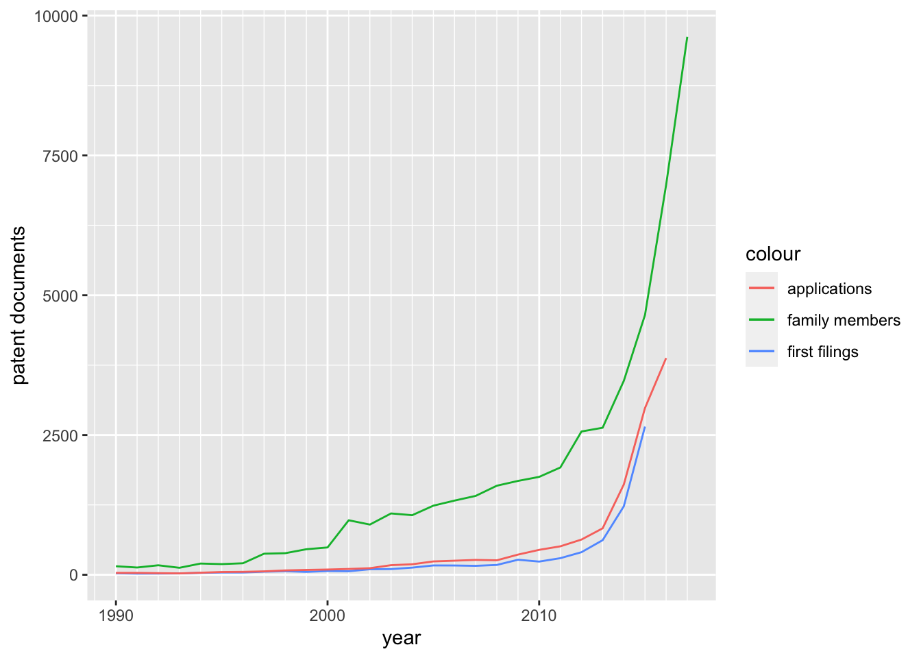
Figure 4.8: Trends in Publications (INPADOC Family Members)

We can see in Figure 4.8 that the difference between the patent publications linked to the applications and the first filings is dramatic. We will consider different definitions of patent families below. For the moment, the important observation here is that trends in the publication of INPADOC family members linked to the applications and priority filings do not closely match the pattern displayed by the applications and priority filings. What we are observing here is the multiplier effect of demand for patent rights in multiple countries around the world.

Demand for patent rights, as manifest in the filing, pursuit and maintenance of patent rights in multiple countries is an expression of the importance of the underlying invention to the applicants expressed in their willingness to pay for the pursuit of patent protection in different jurisdictions. Whereas first filings of patent applications are a proxy indicator for investments in research and development, trends in patent publications are an indicator of the commercial importance of those inventions to the applicants expressed in willingness to pay the relevant fees for examination of applications and the maintenance of patent grants. As we will see below the size of a patent family is therefore an indicator of the importance of an underlying invention to the applicant. However, as we will now see, while the majority of attention in patent statistics focuses on counts of priority filings and applications, publication data provides a route to identifying trends in patent applications and grants on the country and instrument level.

4.6 Trends by Country using Publication Data

In this section we illustrate the process for developing patent trends analysis at the country level using the drones data. However, it is important to emphasise that the drones dataset is not complete. A complete analysis would require the construction of a patent dataset that used searches for relevant jurisdictions in the appropriate languages using tools such as Patentscope CLIR (Cross Lingual Information Retrieval) which facilitates the translation of search terms into other languages. As such the drones data we will be working with is incomplete for national level analysis. However, bearing this limitation in mind, it is nevertheless useful for illustrating methods, considering the issues that are likely to be encountered and how to deal with them.

When seeking to develop analysis on the country level it is important to note that some countries and instruments will display high levels of activity (WO, EP, US, JP, CN and others) while others will display very low levels of activity. As a consequence, attempts to graph the data will results in a large number of countries appearing at the bottom of the graph.

One approach to this is to simply focus on graphing the countries/instruments with the highest number of results. We will focus on mapping trends for the top countries and instruments. Figure 4.9 displays the trends in publications, as an indicator of demand, for the top countries and instruments.

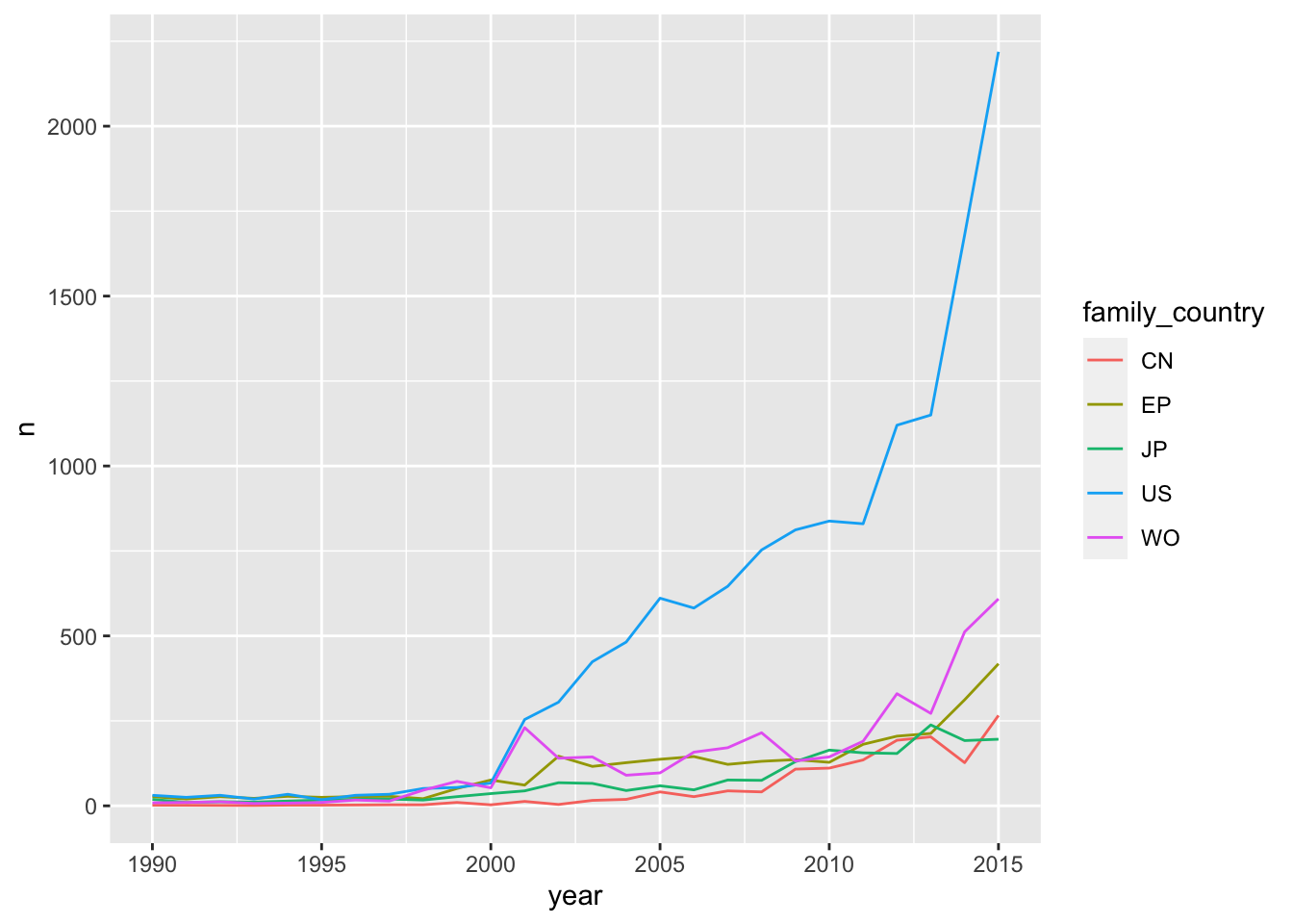
Figure 4.9: Trends in Publications using INPADOC Family data

Figure 4.9 reveals that in terms of patent publication counts the United States is the lead country by a considerable margin, followed some distance behind by the international Patent Cooperation Treaty (PCT with code WO) and the European Patent Convention (EP) administered by the European Patent Office (EPO) and in turn by Japan (JP) and China (CN). Note however, that this is not comparing like with like as the US data is confined to a single country whereas the EP and PCT are vehicles for the pursuit of protection in multiple countries.

We can also see that the dominance of the US data in terms of counts of publications is compressing the data for the other main countries and instruments to the bottom of the graph. In practice, the difference is so marked that we would probably seek to separate out the data. We will address this in greater detail below.

Patent publication data, in this case derived from INPADOC Family Member numbers, is important because it allows for the analysis of trends in patent applications and patent grants using patent kind codes.

As discussed above, one challenge with patent kind codes that describe publication levels is that their use has varied over time. Thus, in the United States prior to 2001 patent documents were only published when granted and received kind code A (first publication level). After 2001 the United States began publishing patent applications as the first publication level and they received kind code A while kind code B is used for the second publication level (granted patents).

This has two impacts on counts of patent data. First, as we see in Figure 4.9 the data for the United States appears to leap between 2000 and 2001. This does not reflect a leap in patent activity but is instead a reporting effect arising from the publication of both applicants and grants. Second, we cannot simply use the A and B kind codes to separate out trends in patent applications and grants for the United States because they refer to different types of publications over time.

To address this we have created a field in the families table called kind-adjusted that has converted US kind code A documents to kind code B in the period before 2001. The original kind code is maintained in a field called kind_original as good practice when transforming the original data.

The effect of this adjustment is shown Table 4.8 where based on the date of the publication (family date), the kind code is adjusted.

Table 4.8: Adjusting historic kind codes for US patent data

family_members	family_date	kind_original	kind_adjusted
US5551521A	1996-09-03	A	B
US5894897A	1999-04-20	A	B
US6158531A	2000-12-12	A	B
US5920995A	1999-07-13	A	B
US6032374A	2000-03-07	A	B
US5155307A	1992-10-13	A	B

Figure 4.10 displays trends in patent applications and grants based on this adjustment.¹⁰

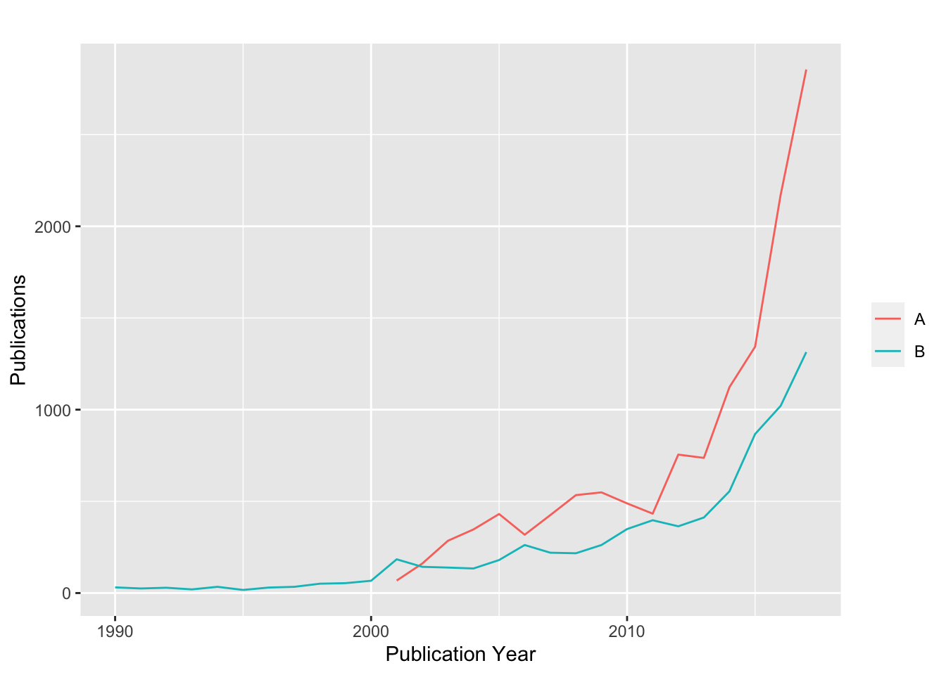
Figure 4.10: Trends in US Patent Applications and Grants

These raw counts of publications with kind code A for applications and kind code B for patent grants reveal two points. In the case of this data there appears to have been a spike in patent grants between 2000 and 2001 from 67 to 184 grants which may, or may not, be associated with the shift to the publication of patent applications from 2001 onwards. The second point is that we observe the start of the publication of patent grants from 2001 onwards with notable peaks and troughs suggesting that this graph would benefit from smoothing. However, for our purposes we can clearly see the point at which US data is transformed in scale by the publication of applications. The important point to bear in mind here is that in the period prior to 2001, US patent activity was under-reported relative to activity elsewhere because only data on grants was published. From 2001 the US harmonises with the rest of the world and we see an apparent jump in activity that is in fact a reporting effect.

In considering the use of patent publication data (in this case arising from INPADOC family members) it is important to remember that data by publications also leans forward. Peaks and troughs in this data will in fact reflect changes in underlying filing activity from at least two years before. In addition, peaks and troughs will be affected by strategic behaviour by applicants such as the filing of continuation, continuation in part and divisional patent applications (see Hegde, Mowery, and Graham 2007 for discussion) along with administrative issues within patent offices that may affect the publication of patent documents.

As this example suggests, significant caution is required when seeking to use publication data to map patent applications and grants in any given country. That is, it is important to investigate the use of kind codes over time for each country that is included in an analysis. For example, in a number of European Patent Convention (EPC) member states, a regional European patent grant only becomes a national patent grant when it is translated. These documents are awarded kind code T. In EPC member states kind code T is therefore equivalent to a patent grant.

We will now look at trends across the top 10 countries. In doing so we need to recall the major caveat that this data will be incomplete for drone technology in each country. However, to get a feel for this we will start simply by mapping trends in publications and then break the data down using kind codes. Because some of the countries in the top ten have relatively limited activity we will include a Loess smoothing trend line rather thank linking the data points. The results are presented in Figure 4.11 and limited to the period 2000-2017 for ease of visibility.

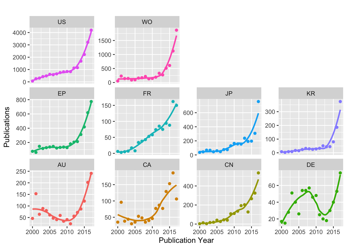
Figure 4.11: Publication Trends for Top Ten Countries (INPADOC Family Members)

In considering Figure 4.11 note that the scale of activity (shown by the y axis for each country) reveals quite dramatic differences in activity for each country. We can also see that Australia (AU) and Germany (DE) display unusual patterns. This type of pattern typically reflects a relative lack of pattern in low frequency data. As such, this type of graph can assist with decision making in identifying the most significant sources of data to present to readers for analysis.

In work on the development of the scientific and patent landscape for marine genetic resources for South East Asian countries a problem emerged where major peaks were encountered followed by zero or very low activity. Radical peaks and troughs in patent data typically suggest missing data. In the case of South East Asia it transpired that the EPO Worldwide Patent Statistical Database (PATSTAT) had very limited coverage of ASEAN national collections and thus presented a very partial view when compared with Derwent Innovation which includes the ASEAN national collections. As such, graphs of the type displayed above should be initially used for exploratory data analysis with a focus on the assessment of the completeness of the data (in this case we know that the data will be incomplete).

Figure 4.11 also provides us with important clues on what we might expect when we seek to visualise patent trends by kind codes for these countries. That is we should expect to see erratic data or no real pattern for countries with lower counts. For illustration Figure 4.12 presents the breakout of the data for each country above using kind code A and B and excluding other types of document (e.g, Utility models and designs). Note that for the purpose of discussion we are ignoring the variations in the uses of kind codes in the countries.

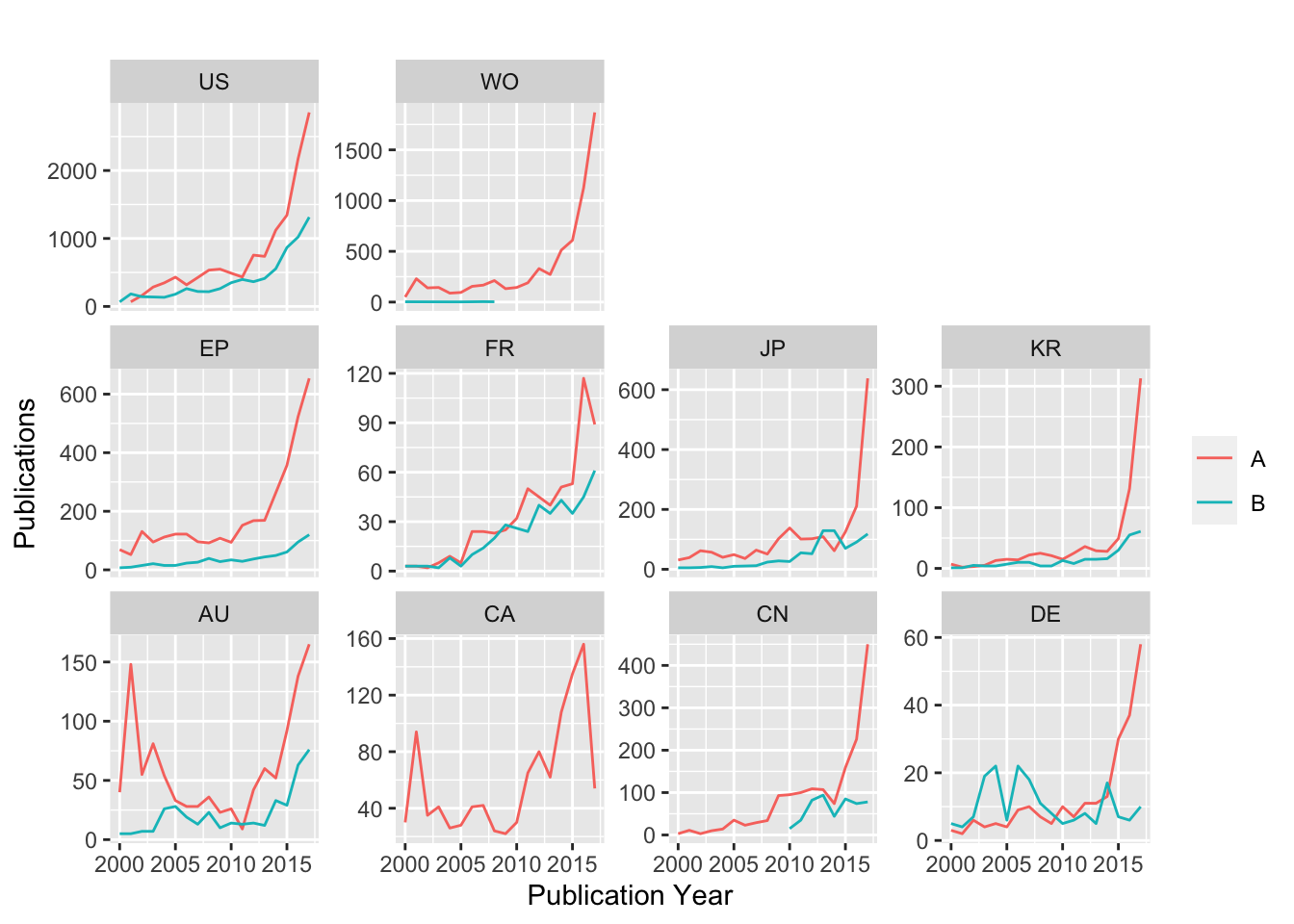
Figure 4.12: Publication Trends for Top Ten Countries with Kind Code A and B

A number of features emerge in Figure 4.12, In the case of the Patent Cooperation Treaty (PCT and coded WO) we can see a small number of patent documents with Kind Code B. In practice there are two PCT documents in the dataset with Kind Code B. This is presumably a data entry mistake because WIPO does not issue documents with Kind Code B as the PCT has no second publication level. A second feature emerges in the case of Japan (JP) where the number of patent applications dips dramatically below the level of B documents before increasing dramatically. We would reasonably expect that the application rate would be higher than the grant rate. In practice, this issue will reflect the incomplete nature of the dataset we are working with.

A third issue arises with Australia (AU) which exhibits a peak in activity around 2000/2001 and then collapses. One known issue with data from Australia is that around this period Australia recorded PCT designations as if they were actual applications leading to distortion of the statistics between approximately 2000 an 2003.¹¹

In the case of Canada (CA) we observe activity for Kind code A but no activity for Kind code B. This illustrates the importance, as emphasised above, of examining the use of kind codes in individual countries that will be the focus for analysis. Canada uses Kind code C for patent grants while Kind Code B is used for reissue patents.

The case of China (CN) which displays data for kind code B from 2010 onwards may suggest that there are limitations in the availability of patent grant data that require investigation. In the case of Germany (DE) this exposes the limitations of our dataset (which did not involve searching the German collection). While bearing this in mind, note that the data on patent grants (which exceeds those for applications) is reflecting the translation of EPC patent grants (with kind code T for Translation). In practice the landscape of Kind Codes for Germany is quite complicated and once again reveals the need to review Kind Codes with considerable care when developing this type of analysis.

4.7 Patent Families

In the preceding sections we have moved from counting patent data by priority or first filings, to counting applications and then using patent publications to explore the issues involved in mapping trends in patent applications and grants on the country level. As we have seen when we move to the country level issues of data capture from the language of the search strategy and the interpretation of kind codes become major issues.

As part of this discussion we used patent publication data from INPADOC Family Members that are linked to the underlying first filings. We will now look at patent families and their uses in more detail.

At its simplest a patent family is a grouping of patent documents based on a relationship or set of relationships. As we will see below that relationship can vary. However, for everyday purposes the following working definition has the benefit of being simple and easy to remember.

At its simplest a patent family can be understood as a stack of documents published in any language anywhere in the world that share a common parent in the form of a priority number.

As we will see, this simple working definition describes around 75% of patent families in the EPO Worldwide Patent Statistical Database (PATSTAT) database.

In practice, there are a number of different definitions of patent families.

1. Simple first filing based families. These are families where members must share a priority number (Martinez 2010a).
2. DOCDB families. Similar to the above except that based on expert review at the EPO documents with the same technical content are added to the family. DOCDB refers to the EPO central documentation database (Martinez 2010a)
3. INPADOC extended families. These families share the DOCDB definition but the definition is expanded so if document A shares a priority number with document B they are in the same family. However, if document C shares a priority with document B but not document A then document C will still be grouped in the family of document A. In addition, examiners may identify other technically related documents that are added to the family. INPADOC patent families are therefore larger than DOCDB simple families (see below).
4. Triadic patent families (OECD definition for filings shared between the US, EP and JP). This is used by the OECD in patent analysis to refer to patent filings that are made in the United States, at the European Patent Office and in Japan. The aim of these families is to allow for analysis of the internationalisation of technology by neutralising the home bias created by the fact that most applications are made in national offices. This is achieved by focusing on those made at the three major offices (Dernis and Khan 2004; Criscuolo 2006; Sternitzke 2009).
5. Derwent Patent families. A type of patent family used in the Derwent World Patent Index from Clarivate Analytics. This type of patent family relies on the identification of new priority filings that become the Basic patent for a patent family. Documents sharing that priority are classified as equivalents and become part of the patent family and includes continuation and continuations in part. In addition, what are called non-convention equivalents that do not share a priority but with the same technical content are added to the family and marked. This allows users to identify documents for the same invention that do not share a priority.
6. PatBase families. PatBase defines its families as follows: “A PatBase family contains all publications that share one or more common priority number(s). This includes continuations-in-part. If PatBase families become very large (100+ members) where possible these are broken down into sub-groups of simple families. A simple family is one where all priority numbers are shared.”

It is likely that this list of definitions of patent families is incomplete but it indicates the range of possible groupings.

In practice, the most commonly encountered definitions of patent families are simple families, DOCDB families and INPADOC extended families.However, as we can see from the definitions above one challenge with patent families is that there appears to be an element of subjective judgement whereby examiners or database providers take decisions on the members of patent families. In addition patent database providers do not always clearly describe the process for determining patent families. This can make patent families confusing and indeed obscure. The simple working definition provided above is designed to help maintain clarity of focus.

Research on patent families has been greatly enhanced by the creation in 2006 of the EPO Worldwide Patent Statistical Database (PATSTAT). In 2010 Catalina Martinez published an important OECD Working Paper entitled Insight into Different Types of Patent Families” on the structure of patent families using PATSTAT data for the period between 1991 and 2009 (Martinez 2010a, 2010b). This study made a major contribution to clarifying the impact of different definitions of patent families using PATSTAT as an international baseline and also explored the structure of patent families. We will now briefly summarise and explore the main findings from this study.

Martinez focuses on the important question of how to build patent families and identifies four types of linkages that can be used to build patent families:

1. Paris Convention priorities
2. Technical similarities (also called non-convention priorities, intellectual priorities or technical relations)
3. Domestic priorities (e.g.continuations, continuations in part, provisionals, divisionals)
4. PCT regional/national phase entries (Martinez 2010: 23)

Each of these types of linkages is accompanied by a definition and whether the information is provided by the applicant as in Table 4.9 reproduced from Martinez below (Martinez, 2010. Table 7, 23)

Table 4.9: Sources of the Building Blocks for Patent Families

Type	Definition	Claimed by applicant in patent document
Paris Convention priorities	Allow a one year delay between first original filing and subsequent foreign filings by same applicant claiming the priority right (1883 Paris Convention).	YES
Technical similarities	Relations among patent documents with similar scope, inventor and applicant names, that nevertheless lack common priority. An artificial priority link is assigned manually by the database producers.	NO
Domestic priorities	Filed at the same office. They are mainly continuations, continuations in part and provisionals (the three of them only available at USPTO), and divisionals, which are available at most patent offices (1883 Paris Convention).	YES
National phase entries of PCT filings	Entry into regional/national phases of PCT filings.	YES

As we can see in this table, the source of information for building patent families predominantly comes from the applicant except for the technical similarities. Technical similarities are identified by examiners based on their assessment of the scope, inventor and applicant names and lead to the creation of an artificial priority link. As such, the identification of technical similarities is not purely subjective.

Martinez then uses the EPO Worldwide Patent Statistical Database (PATSTAT) to quantify the impact of the use of the different linkages on the size of patent families for the period 1991 to 1999. Table 4.10 reproduces Table 9 from Martinez’s research.

Table 4.10: Counts of families and applications in them, by source of family relations 1991-1999 (Martinez 2010a)

	Source 1 Families		Source 2 Families		Source 3 Families		Source 4 Families
	Paris Convention		Paris Convention + Domestic Continuations		Paris Convention + Domestic continuations + Technical similarities)		Paris Convention + Domestic continuations + Technical similarities + PCT national phase entries
year	families_1	members_1	families_2	members_2	families_3	members_3	families_4	members_4
1991	106850	567024	110371	610367	110856	614631	110745	614888
1992	107873	571499	113659	624205	114394	629235	114276	629538
1993	112351	602058	119014	655380	119656	659896	119533	660106
1994	116602	639485	123818	693431	124606	698404	124362	699194
1995	129535	722318	135946	761371	136702	766020	136405	766939
1996	146281	805300	152088	849307	152994	854422	152681	855240
1997	161060	874480	166277	914281	167220	919518	166857	920284
1998	173243	939352	179345	985989	180095	990508	179618	990914
1999	196972	1057368	204330	1102833	205222	1106929	204659	1107482
1991-1999	1250767	6778884	1304848	7197164	1311745	7239563	1309136	7244585

Note that Table 4.10 focuses on the earliest priorities and excludes singletons.b A number of important points emerge in Martinez’s analysis. The first of these is that “Paris Convention priorities alone make up more than 95%, which make them the most relevant patent linkage by far in the construction of extended patent families.” As such Paris Convention priorities are the foundation of patent families.

The second major observation is that the number and size of families increases as the definition is expanded in the first three cases. The third case exactly matches with the widely used INPADOC extended patent family definition (Paris, domestic continuations and technical similarities). However, observe that the number of families in the final case in the table is lower in all cases than for the source 3 (INPADOC) even while the number of family members increases. The reason for this is that first three types create new independent families. In contrast, the final type consolidates families by revealing shared links through the Patent Cooperation Treaty. That is, the number of families falls because otherwise hidden linkages with the PCT become obvious (see Martinez 2010: 25).

Using this data we can visualise the impact of different types of counts of families and family members. We will focus here on displaying the difference between the simple family definition and the INPADOC definition (source 3 above). Figure 4.13 trends in the number of patent families using the simple and INPADOC definitions (Martinez 2010a).

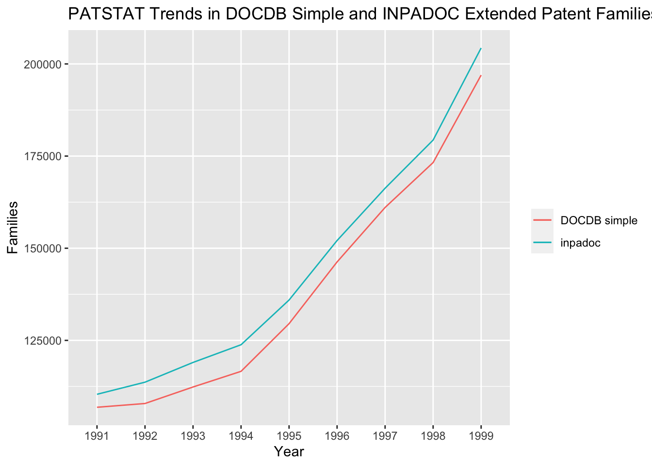
Figure 4.13: PATSTAT Trends in DOCDB Simple and INPADOC Extended Patent Families

We can see here that the DOCDB simple families and the INPADOC family counts follow the same pattern except that the number of INPADOC families are consistently larger than the DOCDB simple families.

Figure 4.14 places counts of the number of families and the number of family members onto the same graph. This brings the difference between counting the number of families rather than the number of family members into focus.

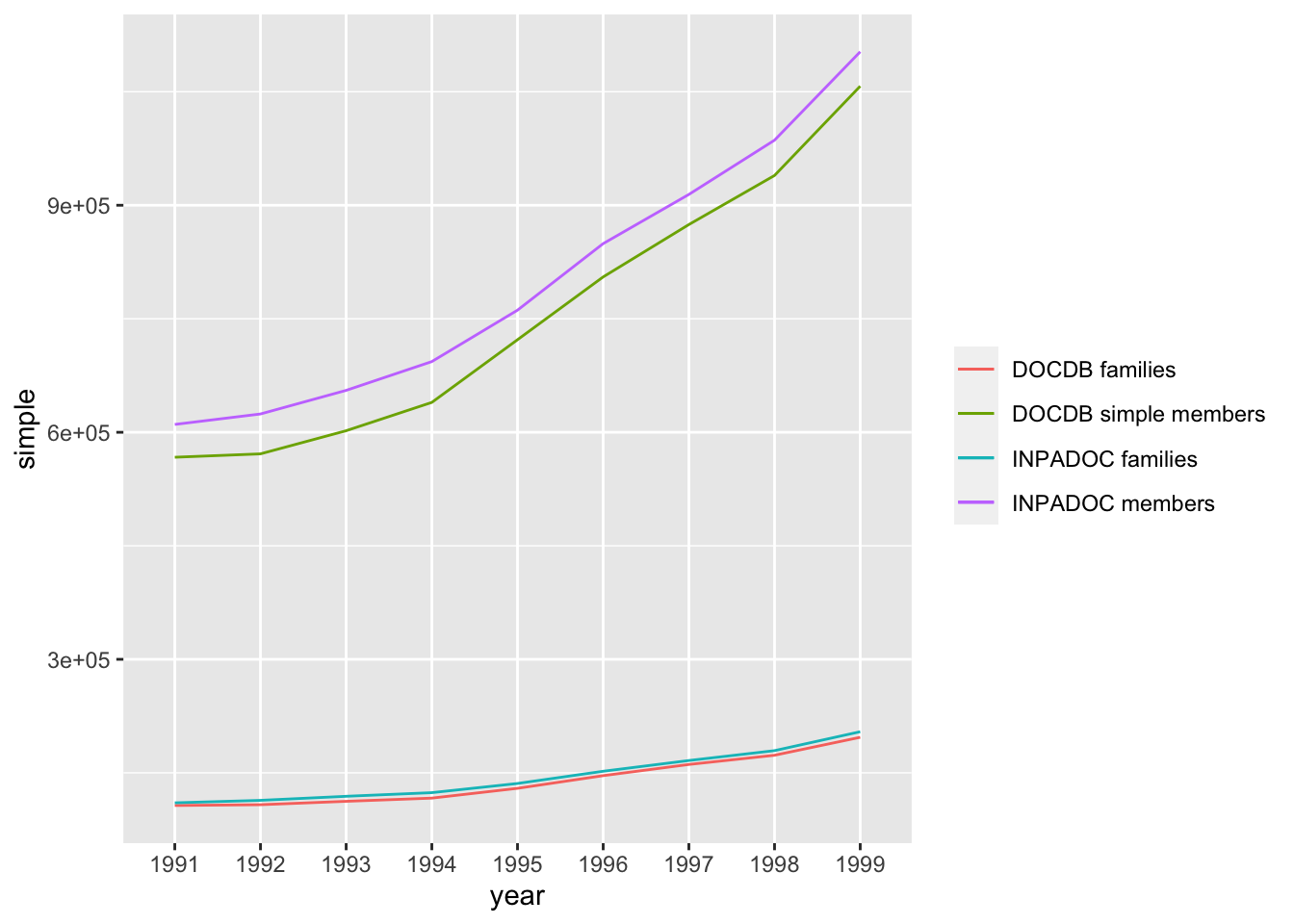
Figure 4.14: Trends in Patent Families (priority filings) and Family Members compared

In considering this graph note that while the families count range is in the hundreds of thousands, with 205,222 INPADOC families in 1999, the equivalent count for INPADOC family members was 1,106,929. Under both the DOCDB families and the INPADOC families definitions this brings home the scale of the multiplier effects arising from the publication and republication of patent documents. We have seen a similar type of pattern in Figure 4.8 for the drones data where the number of patent family members accelerates away from the priority filings as publications multiply.

Martinez also explores and quantifies the different structures of patent families in the period between 1991 and 1999 (see in particular Martinez 2010a). Martinez developed an algorithm to assess the structure of the INPADOC patent families discussed above and found that:

“Applying the algorithm just described to the 1 311 745 INPADOC extended patent families with earliest priorities in the 1990s, as reported in PATSTAT September 2008, and excluding families formed by one patent document only (singletons), a total of 47 437 different family structures are identified. Among them, however, only a few structures are really popular: 86% of the structures represent just one family each, whereas only 10 structures represent 73% of all families and 25 represent 81%. In addition, more than half of the top 25 structures are made up of one earliest priority followed by several direct subsequent filings, what we will call “simple structures” from now onwards.” ¹²

The important point here is that while initially the structure of patent families may appear to be extremely diverse, with 47,437 different family structures, in practice 10 structures described 73% of the families and 25 structures accounted for 81%. This is a very significant finding because it informs us that the majority of the time the structure of patent families falls within a limited set. Furthermore, of the top 25 structures, over half are made up of a simple structure consisting of a single earliest priority followed by several direct filings. Martinez goes on to conclude that “…we have found that 75% of all INPADOC extended priority patent families with earliest priorities between 1991 and 1999 have a simple structure, consisting of one single first filing and its direct subsequent filings” (Martinez 2010a). The broader significance of this is because INPADOC extended families are the broadest category of common family types that 75% of other patent families will be of the single first filing and direct subsequent (child) filing type.

From this we can reasonably conclude that the majority of patent families that we will ever encounter will be of the simple type (single priority followed by several direct filings). However as Martinez also notes “Complex families may favour specific technologies, countries or more valuable patents” (Martinez 2010: 17) so it is important to bear in mind that complex families while representing a much smaller proportion of the data may also be important when dealing with particular fields or valuable patent families.

In considering the use of different types of family counts the most commonly encountered forms will be the DOCDB simple family types or the INPADOC family types. In the sections above we have graphed families (priority filings) and used raw family members to explore trends in different countries. However, as mentioned above the size of patent families is an indication of the importance of an invention to the applicants based on their willingness to pay fees for the stages of the procedure and for the maintenance of any granted patents in one or more jurisdiction. Table 4.11 displays the raw count of INPADOC family members across the drones dataset linked to the earliest priority number.

Table 4.11: Top INPADOC Families

earliest_priority	application_number	family_count
AU19977991A 1997-07-15	JP200944799A 2009-02-26	2964
US13420236A 2012-03-14	US14253376A 2014-04-15	1819
US2013811981P 2013-04-15	US14253099A 2014-04-15	1819
US2001270625P 2001-02-23	EP2002714961A 2002-02-21	1440
US2011452418P 2011-03-14	US14024204A 2013-09-11	808
US2002387792P 2002-06-11	US13602510A 2012-09-04	808
US14064189A 2013-10-27	US14526503A 2014-10-28	371
US13158372A 2011-06-10	US14065419A 2013-10-29	371
US201364189A 2013-10-27	EP2014857043A 2014-10-28	371
US14065415A 2013-10-28	WO2014US62477A 2014-10-27	371

The top result in the drones dataset lists an earliest priority filing in 1997 and concerns Methods for Manufacturing Inkjet Print Head using Multilayer Material Layer by Silverbrook Research in Australia involving Kia Silverbrook who has been described on Wikipedia as having been the worlds most prolific inventor.¹³ According to news reports Silverbrook Research went into administration in 2014.¹⁴.

This is an example of noise in our drones dataset and a historic example, however the size of the INPADOC patent family indicates that the claimed invention was of great importance to the applicants. Table 4.12 displays the countries that have been the focus for the development of this family. Note that each document in the family is counted.

Table 4.12: Top Family Countries for priority AU19977991A

family_country	raw	consolidated
US	2116	2116
AU	334	292
SG	52	52
EP	119	49
JP	44	44
WO	40	38
CN	35	35
DE	38	31
IL	55	30
KR	30	30
AT	28	28
ZA	27	27
CA	43	26
NZ	2	2
ES	1	1

Table 4.12 shows the raw counts of family member documents for each country and the consolidated counts (with the kind codes removed to group by document identifier). The documents are ranked on the count of the consolidated family members.

We can immediately see that while the applicant company was Australian the key target market was the United States followed by Australia, Singapore, Europe (through the European Patent Office) and Japan. By far the greatest intensity of family members is found in the United States and it transpires that these family members are clustered by date. Figure 4.15 shows US family member publications as a simple frequency plot over time.

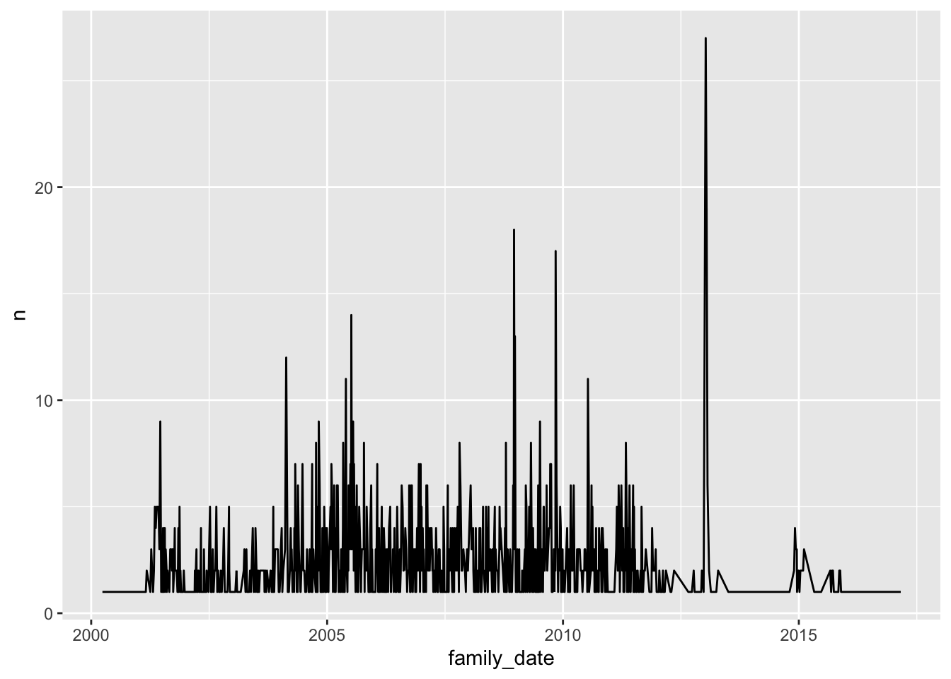
Figure 4.15: Frequency Plot for the Publication of US Family Members for priority number AU19977991A 1997-07-15

Figure 4.15 shows a strong clustering effect. In order to more clearly understand what is happening inside this plot Figure 4.16 displays the frequencies for US granted patents within the family over time (kind code B).

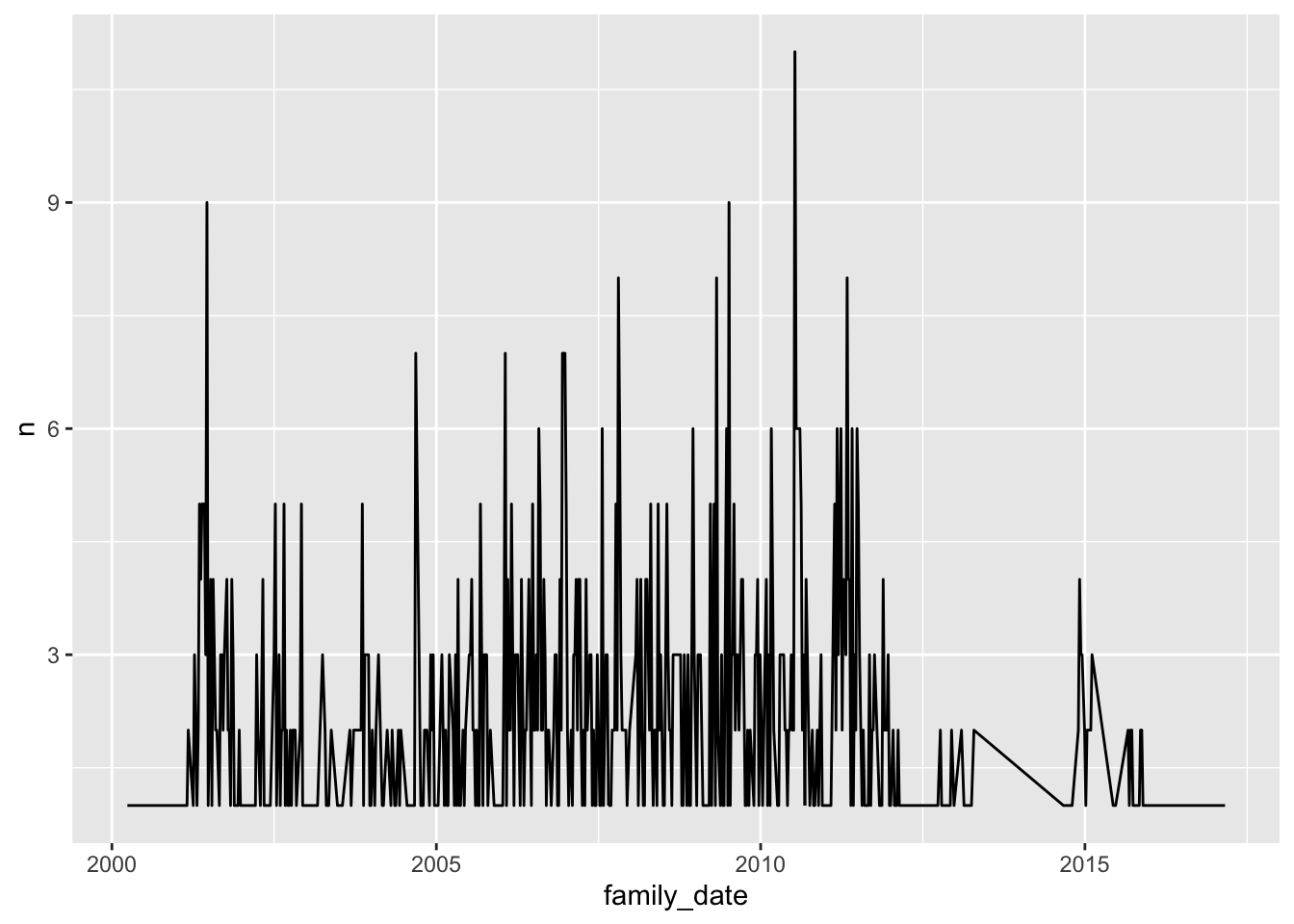
Figure 4.16: Frequency Plot for Patent Grants among US Family Members for priority number AU19977991A 1997-07-15

What emerges here is that there are 1,086 US patent grants that can be traced to the single Australian priority filing.¹⁵ The earliest US patent grant in the set was published in March 2000 as US6041600A for the Utilization of quantum wires in MEMS actuators that claims priority to the Australian document. The latest patent grant in 2017 provides the explanation for what has been happening with the family members.

The text of the most recent patent grant US9584681B2 for a Handheld Imaging Device Incorporating Multi-Core Image Processor in the description on related applications says:

This application is a continuation of U.S. application Ser. No. 13/101,131 filed May 4, 2011, which is a continuation of U.S. application Ser. No. 10/656,791 filed Sep. 8, 2003, issued Jun. 7, 2011, as U.S. Pat. No. 7,957,009, which is a continuation application of U.S. application Ser. No. 09/922,274 filed Aug. 6, 2001, issued Sep. 9, 2003, as U.S. Pat. No. 6,618,117, which is a continuation-in-part application of U.S. application Ser. No. 09/113,053, filed Jul. 10, 1998, issued Mar. 26, 2002, as U.S. Pat. No. 6,362,868. Each of the above identified patents and applications and U.S. Pat. No. 6,238,044 are hereby incorporated herein by reference in their entirety.

While we have not been able to review the entire portfolio of patent grants, a review of the five most recent documents suggests that the US members of this family have been constructed from a long series of continuation and continuation in part applications.

Further analysis of this specific case is beyond the scope of the Handbook. However, as discussed in the recent in depth review of patent family research by Dechezleprêtre et. al. 2017 it highlights the strategic uses of the patent system with respect to continuation filings (Dechezleprêtre, Ménière, and Mohnen 2017). Lemley and Moore provide a critique of the use of continuations in the US system and focus on the extreme example of patent activity by an individual inventor (Jerome Lemelson) in connection with bar code readers (Lemley and Moore 2003). They highlight that by using continuations and continuations in part:

“Inventors can keep an application pending in the PTO for years, all the while monitoring developments in the marketplace. They can then draft claims that will cover those developments. In the most extreme cases, patent applicants add claims during the continuation process to cover ideas they never thought of themselves, but instead learned from a competitor. The most egregious example is Jerome Lemelson, who regularly rewrote claims over the decades his patents were in prosecution in order to cover technologies developed long after he first filed his applications. Lemelson filed eight of the ten continuation patents with the longest delays in prosecution in our study. Those Lemelson patents spent anywhere from thirty-eight to more than forty-four years in the PTO.” (Lemley and Moore 2003)

As Dechezleprêtre et. al. point out the aspects of US patent law that facilitated the specific strategic behaviour by this applicant have been abolished. However, continuations and continuations in part continue to feature as part of the US patent system.

From the perspective of patent analytics, this example demonstrates that we are able to move from the use of patent family data to explore patent activity linked to a priority filing or set of priorities anywhere in the world. We are also able to identify the top ranking patent families and to explore the details of those families in individual countries. Simple techniques such as the use of a frequency plot over time help us to identify patterns in activity. In the case of Silverbrook we have seen that while the company reportedly went into administration in 2014, with a collapse in US family activity observable in the frequency plots above for that period, we then observe the issuance of patent grants from 2015 into 2017 (the end of our data). This suggests that this portfolio has been taken over (perhaps through the sale of the IP to a third party). To proceed further in the analysis of this case we would want to look at the legal status for the documents in the portfolio. Thus, a review of the legal status for the most recent patent grant US9584681B2 reveals that it is now owned by Google.¹⁶ In addition, as discussed by (B. H. Hall and Harhoff 2012) the analysis of patent renewal fees has an important role to play in analysis of the economic value of patent grants within a family portfolio.

The discussion of patent families presented above points to the richness of research that is possible using patent family data. It is important to note that different definitions of patent families are important in patent analytics and may yield different insights. Thus, one criticism of INPADOC patent families is that they are too broad and a simpler more focused definition may be preferred. In other cases as in the work by the OECD the use of trilateral patent families is intended to promote international comparability by removing the home bias in patent data. The use of this type of definition is important for both comparability and identification of more important patents. Thus, in the case of countries such as China, where filings are heavily focused on the national level, the selection of patent families with international members can facilitate the analysis of cases where Chinese inventors and applicants may be seeking to invest in external markets.

In closing this discussion it is important to emphasise that patent families continue to be a very active focus of research in economics and innovation studies. As the most recent review of the literature by Dechezleprêtre et. al. 2017 has highlighted to date the main focus in this literature has been on using family size as the indicator of value (focusing on the number of countries represented in a family) the number of filings in the priority country along with the time span between the first and last filings within a family also offer insights into patent value (Dechezleprêtre, Ménière, and Mohnen 2017). As such, the discussion presented above presents a starting point for engaging with this increasingly rich literature.

4.8 Modelling Data

So far in this chapter we have focused on practical issues that need to be considered in counting patent data. We now turn to a basic introduction to modelling data as a basis for introducing forecasting techniques. Our aim is not to provide an in depth consideration of modelling, that would require more in depth engagement with statistical concepts and techniques. Rather, we wish to encourage you to engage with modelling. In approaching there topics we should bear in mind that most patent analysts and data scientists are not statisticians or economists. However, many within the data science community are aware of this. As a result there are many resources out there to make these methods and techniques accessible for people who may have very different levels of knowledge and experience with statistics. If you are already familiar with statistical methods you may want to skip to the next section on forecasting patent data.

In this section we focus on two widely used models for linear regression: simple linear regression and loess smoothing (Local Polynomial Regression Fitting). These models are methods for finding the ‘line of best fit’ to represent trends in a set of data points and they are widely used in software tools such as Excel and Tableau among others. We will use these models as an easy way in to modelling data and means for assessing data.

There are many textbooks that address modelling and linear regression for readers of all levels of experience. For R and Python users there is the accessible Practical Statistics for Data Scientists by Peter Bruce et al. For R users seeking a more in depth but accessible introduction to the maths with worked examples there is Discovering Statistics Using R by Andy Field, Jeremy Miles and Zoe Field. More advanced users are likely to benefit from An Introduction to Statistical Learning with Applications in R by Gareth James et al. which builds on the now classic, and maths intensive, The Elements of Statistical Learning: Data Mining, Inference and Prediction by Trevor Hastie et al. The tidymodels framework in R brings together many popular modelling packages in R for intermediate and advanced users.

4.8.1 The Data

WIPO makes its patent statistics available as part of the intellectual property statistics section of its website through the WIPO IP Statistics Data Center. Under the PCT section of the Data Center we are able to select a range of indicators. For our purposes we select PCT applications by filing date and Yearly Statistics as the Year Type (note that monthly is also available). A range of different offices around the world can receive Patent Cooperation Treaty (PCT) applications because it is the international patent instrument for submitting applications outside ones home country. We want the number of applications submitted directly to WIPO as the International Bureau and so we choose the International Bureau as the Receiving Office. For simplicity we just choose the Total as the Origin Office.

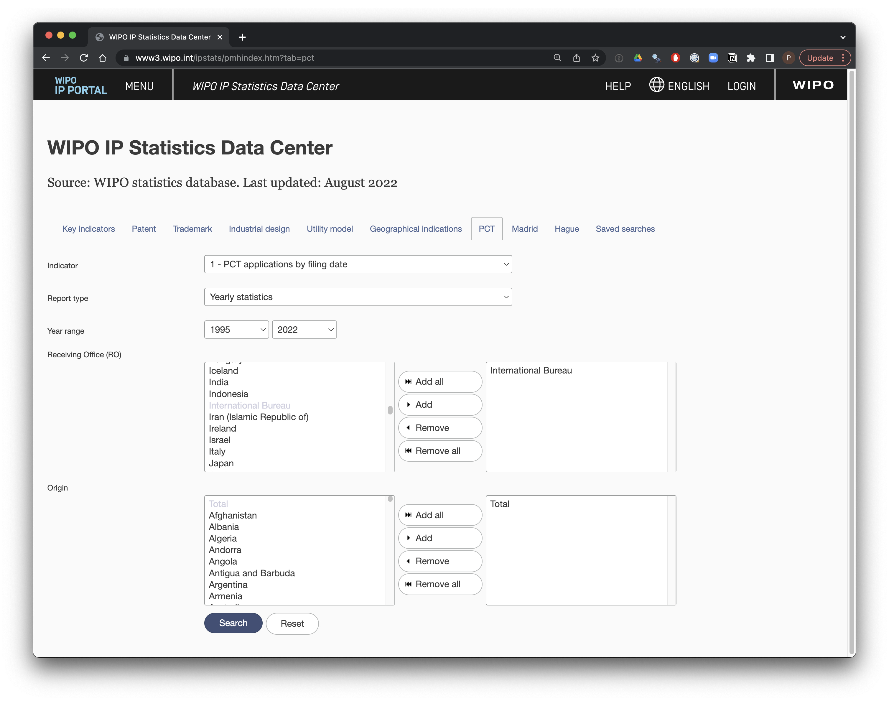
Figure 4.17: Selecting PCT Applications to the International Bureau

When we press Search we see the data that we are after.

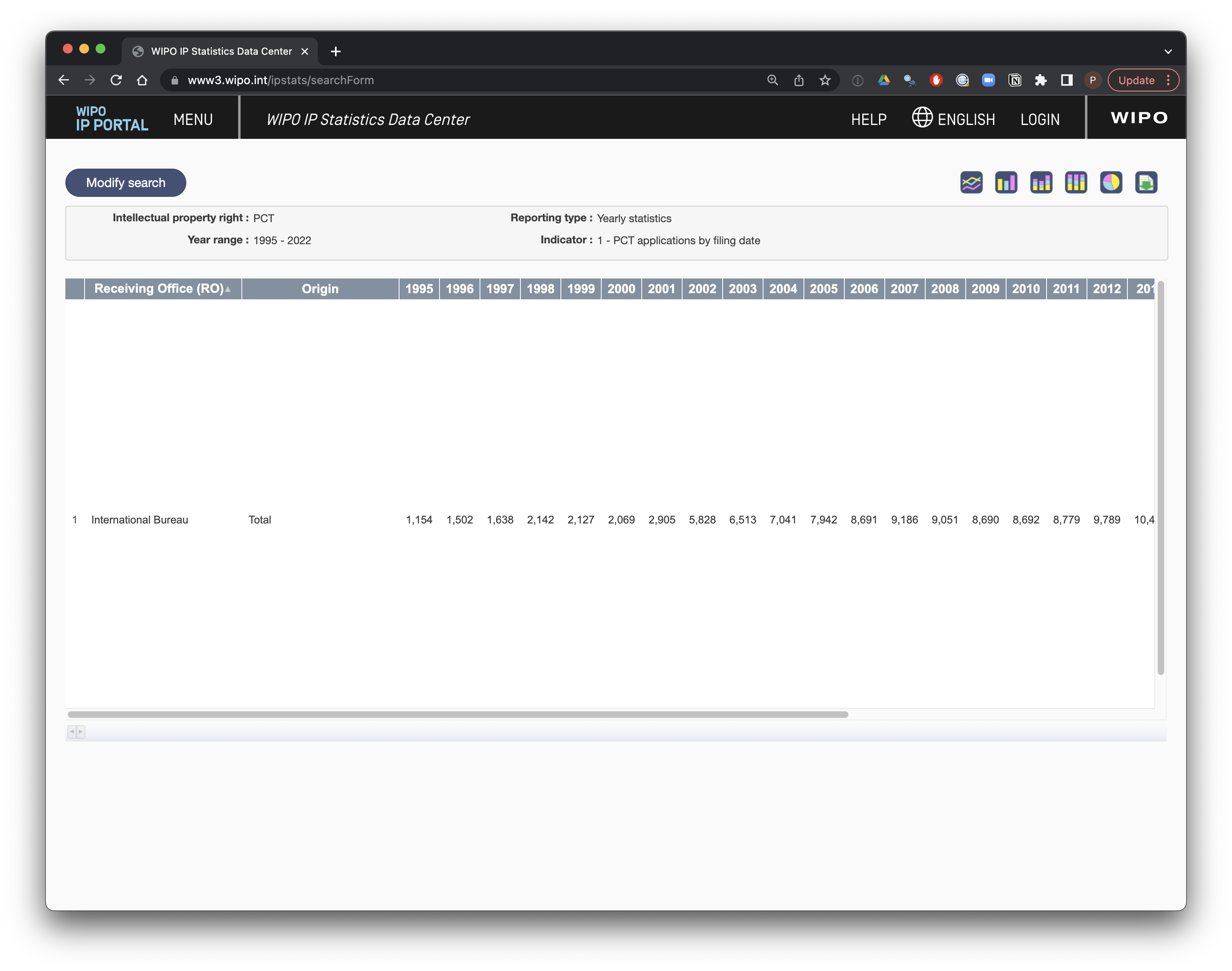
Figure 4.18: WIPO Patent Statistics Data format

Seeing the data immediately tells us something about an initial task before we can get to modelling. The data is in wide format (the easiest for a human to simply print out and read). However, we will want this data in long format with year as the column heading.

Having downloaded the data we start to think about importing into R or Python. However, it turns out that there are some extra headings at the top (which we can normally skip), but more importantly that the heading for the Receiving Office and the Origin columns are on different rows to the year. That requires a frustrating manual fix. When we import the data we discover that the year columns are preceded by an x for reasons that are completely unclear. We make the adjustments and pivot the table to long format. For 2022 the value is not available (NA) and so we simply drop it. This is the reality of data science. Following the manual step we can perform the rest of the transformations with R or Python as we see in the code below.

library(tidyverse)
library(tsibble)
library(slider)
library(fable)

# manually prune uneven rows at the top
# make column names consistent with janitor

pct_ib <- read_csv("data/wipo2022/pct_ib.csv") %>% 
  janitor::clean_names()

# replace junk on import
pct_names <- names(pct_ib) %>% 
  str_replace(., "x", "")

names(pct_ib) <- pct_names

# convert from wide to long format
pct_ib <- pct_ib %>% 
  pivot_longer(., cols = 5:32, names_to = "filing_year", values_to = "n") %>% 
  drop_na(n)

load("data/patent_counts/pct_ib.rda")

We are now in a position to start creating basic models for our data. We will start with a technique that we have already seen in Figure 4.11 above, with the application of a linear model to find the line of best fit between a set of data points using linear regression. Linear regression involves estimating the relationship between what is called a dependent or response variable and one or more independent or predictor variables wikipedia. In R and other software packages, the ability to create simple linear models is commonly built in because their use is so common. In R we can use lm() to create linear models of various types.

We can get a glimpse of our PCT filings to the International Bureau data in Table 4.13.

Table 4.13: PCT applications with the International Bureau

filing_year	n
1995	1154
1996	1502
1997	1638
1998	2142
1999	2127
2000	2069

We then create a set of plots for this data and create two linear models, one with simple lm() and one with loess smoothing as in the code below. The popular R graphing package, ggplot includes methods for displaying linear models as part of graphics. We will create the models directly below.

To move through this process we show four panels in Figure 4.19. In the first panel we see a standard scatter plot. In the second panel we show a line graph that joins the dots. In the third panel we apply a linear model that projects a straight line through the data as ‘the line of best fit’. In the fourth panel we use a form of linear model called loess for what is variously called “locally estimated scatter plot smoothing” and Local Polynomial Regression Fitting.

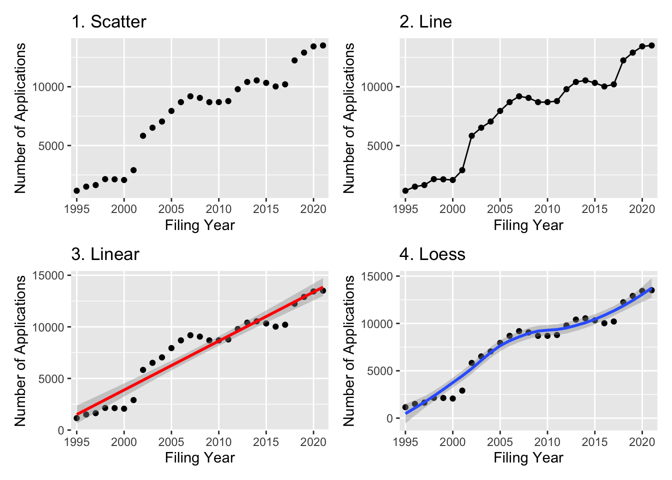
Figure 4.19: Plotting PCT Applications to the International Bureau

In Figure 4.19 we can see that the line plot in panel 2 simply traces a straight line between the data points found in Panel 1. This is the type of graph we commonly see in patent analytics. Panel 3 models a straight line of best fit that passes through the data points. Note how this line reveals positive and negative variation in the data points exposing dips and crests.

In Panel 3 the line of best fit is calculated using the least square method that seeks to mininimse the square of errors between the data points in order to find the best fit. In practice, this focuses on minimising what are called the resiudals between the observed values and the value predicted by the model. Residuals are another name for the standard deviation from the mean.

We can create our linear model directly in R using the lm() function. Here for convenience we use the modelr (Wickham 2022) package to create the linear model and loess model. We start with the lm() model which uses Ordinary Least Squares (OLS) to fit the data by modelling the relationship between the predictor variable (in this case the filing year) and the response value (in this case n for the number of application years to the International Bureau).

library(modelr)

# filing year as numeric

pct_ib <- pct_ib %>% 
  select(filing_year, n) %>% 
  mutate(filing_year = as.integer(filing_year))

# create a model
pct_model <- lm(n ~ filing_year, data = pct_ib)

pct_fitted <- pct_ib %>% 
  add_predictions(pct_model) %>% 
  add_residuals(pct_model) 

pct_plot <- pct_fitted %>% 
  ggplot(aes(x=filing_year, y=pred)) + geom_line() +
  geom_point(aes(y=n)) +
  labs(title="1. Prediction", y="Applications", x = "Filing Year") +
  scale_x_discrete(breaks=seq(1995, 2021, 5))
  
pct_resid <- pct_fitted %>% 
  ggplot(aes(x = filing_year, y = resid)) + 
  geom_point() +
  labs(title="2. Residuals", x = "Filing Year")

pct_compare <- ggplot(pct_fitted, aes(x = filing_year, y = n)) +
  geom_segment(aes(xend = filing_year, yend = pred)) +
  geom_point() +
  geom_point(aes(y = pred), shape = 1) +
  labs(title="3. Predicted and Actual", y = "Applications", x = "Filing Year")

(pct_plot + pct_resid) /
  pct_compare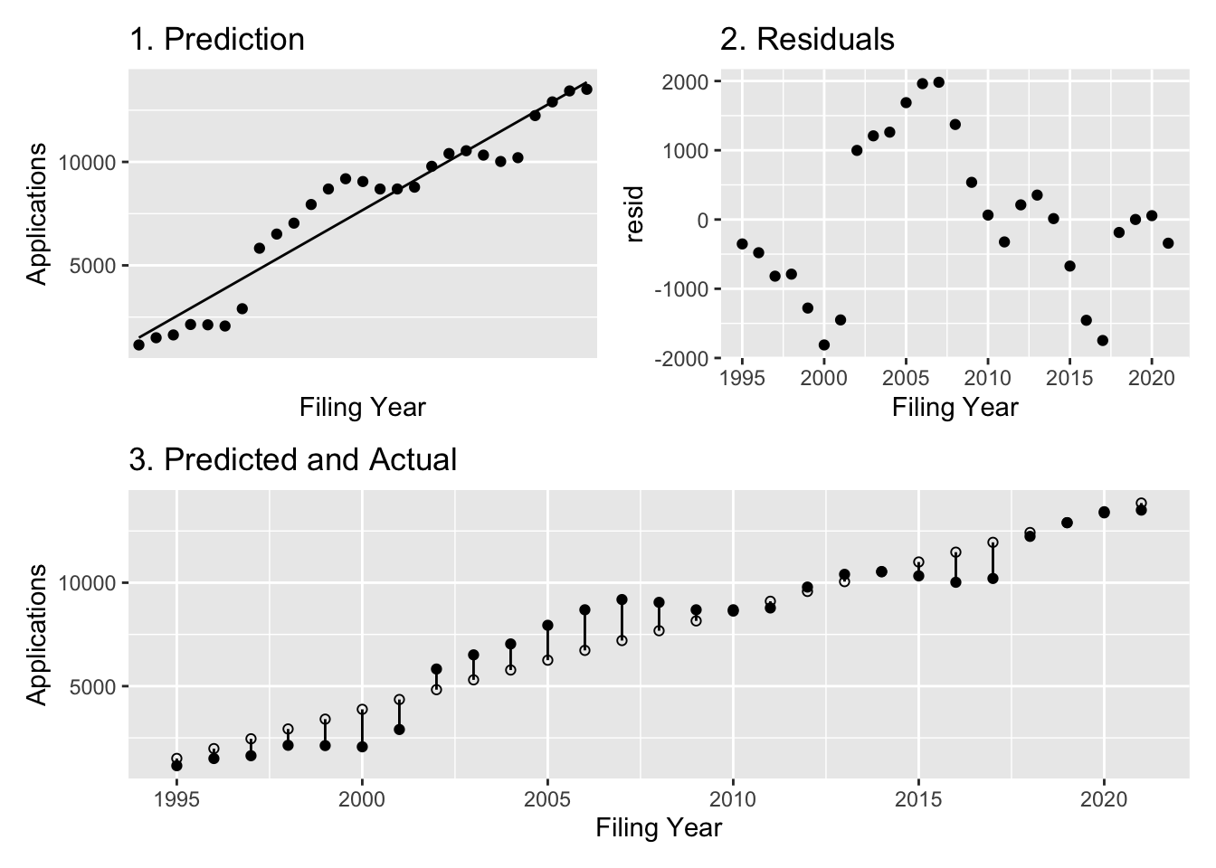

An important feature of regression models and the description of these models is that the data should be normally distributed (that is evenly distributed) around the mean. In reality, a lot of real world data is not normally distributed and displays considerable variation such as outliers. In other words, real world data is often skewed in a variety of ways. In many cases this may not actually matter. Where it does matter is if a specific regression test assumes or requires normality.

Where plotting in this way, notably of the residuals, really helps us is in appreciating the scale of variation. Thus we can observe a trough in 2000 and a peak of filings in 2005-2007, prior to a smaller trough followed by a larger trough in 2016 to 2017. The reader will perhaps already have a sense of the reason these troughs might exist. Other popular ways of visualising this data is in a histogram (see below).

For more detailed analysis than is offered here the summary of the model data is an important starting point for the application of a range of different tests and methods that can be used to both evaluate different models. As a general rule of thumb the a better model is one with lower residuals and error scores.

summary(pct_model)

## 
## Call:
## lm(formula = n ~ filing_year, data = pct_ib)
## 
## Residuals:
##      Min       1Q   Median       3Q      Max 
## -1811.45  -730.79     0.41   767.45  1982.34 
## 
## Coefficients:
##               Estimate Std. Error t value Pr(>|t|)    
## (Intercept) -945607.95   55754.27  -16.96 3.17e-15 ***
## filing_year     474.74      27.77   17.10 2.63e-15 ***
## ---
## Signif. codes:  0 '***' 0.001 '**' 0.01 '*' 0.05 '.' 0.1 ' ' 1
## 
## Residual standard error: 1124 on 25 degrees of freedom
## Multiple R-squared:  0.9212, Adjusted R-squared:  0.9181 
## F-statistic: 292.3 on 1 and 25 DF,  p-value: 2.631e-15

4.8.2 Loess Smoothing

We can appreciate from this that the standard linear model is not doing a great job because of the distribution of the residuals. Our second model, Loess smoothing or Local Polynomial Regression Fitting, uses weighted least squares with subsets of the data from local neighbours to build up the model. Historically, this was more computationally intensive than the standard lm model but is now trivial to calculate.

In the code below we follow the same process that was used above to create and then plot a model using the loess method. In Figure 4.20 we show the prediction from using Loess smoothing along with the residuals and the actual vs. predicted values from the model.

pct_ib <- pct_ib %>% 
  select(filing_year, n) %>% 
  mutate(filing_year = as.integer(filing_year))

# create a model
pct_loess <- loess(n ~ filing_year, data = pct_ib)

pct_l_fitted <- pct_ib %>% 
  add_predictions(pct_loess) %>% 
  add_residuals(pct_loess) 

pct_l_plot <- pct_l_fitted %>% 
  ggplot(aes(x=filing_year, y=pred)) + 
  geom_line() +
  geom_point(aes(y=n))

pct_l_resid <- pct_l_fitted %>% 
  ggplot(aes(x = filing_year, y = resid)) + 
  geom_point()

pct_l_compare <- ggplot(pct_l_fitted, aes(x = filing_year, y = n)) +
  geom_segment(aes(xend = filing_year, yend = pred)) +
  geom_point() +
  geom_point(aes(y = pred), shape = 1)

(pct_l_plot + pct_l_resid) /
  pct_l_compare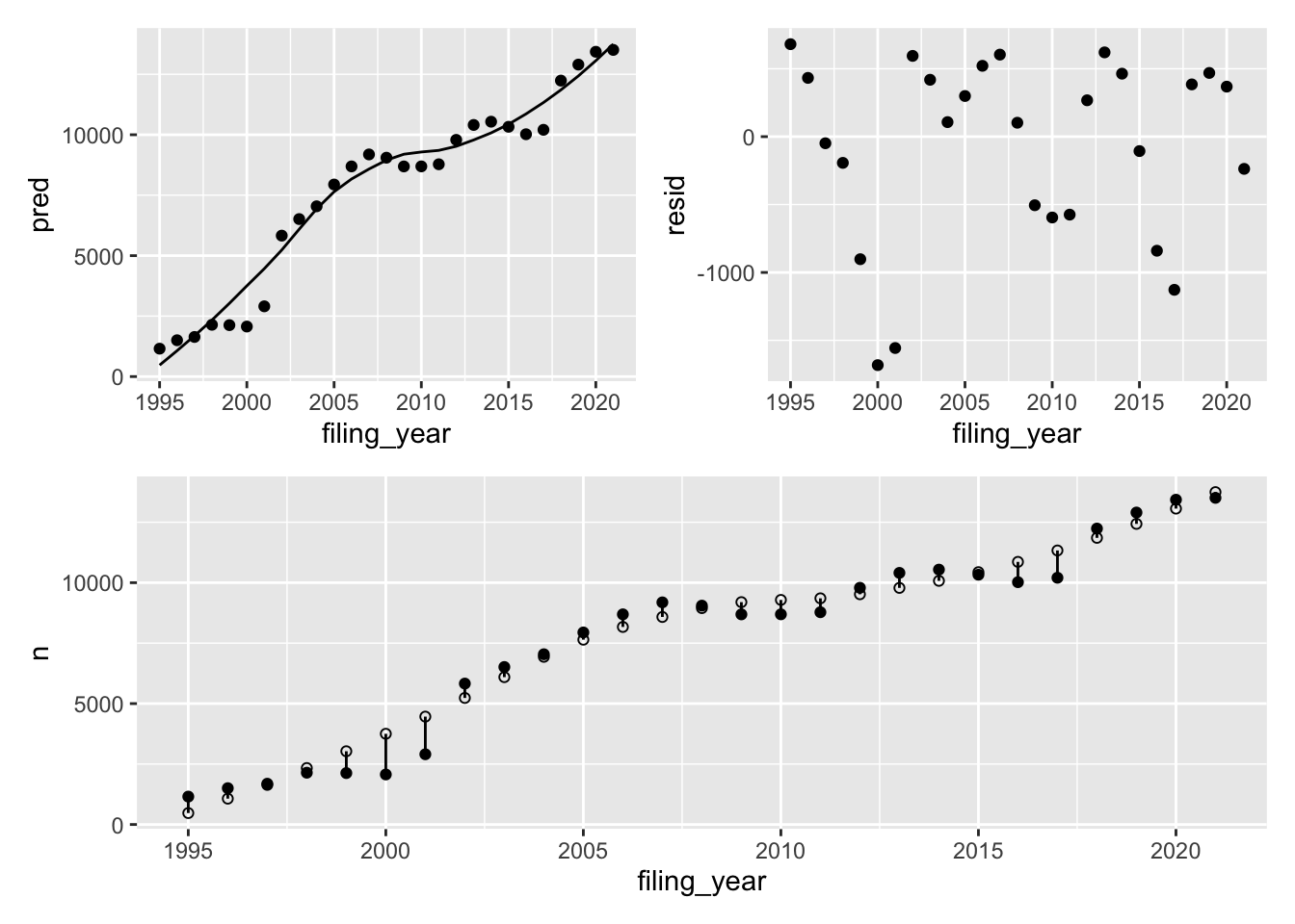

Figure 4.20: Loess Smoothing Results

summary(pct_loess)

## Call:
## loess(formula = n ~ filing_year, data = pct_ib)
## 
## Number of Observations: 27 
## Equivalent Number of Parameters: 4.39 
## Residual Standard Error: 748.4 
## Trace of smoother matrix: 4.81  (exact)
## 
## Control settings:
##   span     :  0.75 
##   degree   :  2 
##   family   :  gaussian
##   surface  :  interpolate      cell = 0.2
##   normalize:  TRUE
##  parametric:  FALSE
## drop.square:  FALSE

On balance in comparing the results of the two models we can see that the Loess smoothing does a better job of fitting to the data because the pattern of the residuals exhibits a narrower range and is closer to zero across the range with the exception of break points representing troughs at 2000, 2008-2011 (to a lesser degree) and 2016-2017. In addition, as the general rule of thumb is to minimise the error we would in this case prefer the lower Residual Standard Error (RSE) of 748.4 from Loess over 1124 from the standard lm model.

In practice, these are only two of the linear models that can be applied to data using R’s lm function (which uses QR decomposition as the method). Other available methods include: robust linear model (rlm), general linear model (glm) and generalized additive model (gam). Some of these, notably gam, come in a variety of flavours and allow you to test and create models for the best fit for your particular data.

Our purpose here has been to introduce these possibilities, and the basic means available for understanding their outputs. As we can see, key features of the use of these models are the analysis of residuals and a range of statistical tests to facilitate comparison between the results produced by different models. We have just scratched below the surface of these models. However, the use of simple linear models is enough of an introduction to grasp some of the key issues involved in one of the most important uses of statistical models: forecasting.

4.9 Forecasting

To conclude this chapter we will briefly introduce forecasting techniques using a fictional situation. Forecasting the future involves a combination of values for time (year, quarter, month, day etc.) and observations for a variable where you want to predict future values for that variable over a time horizon.

Forecasting using time series data matters in many different areas of life because predictions about the future can be incorporated into planning. A great deal may be at stake, for example when trying to predict the stock market or model patient admissions to hospitals during a pandemic.

As we will see below, forecasting is normally based on past observations of a particular variable and the application of statistical methods, notably smoothing, rolling averages and tests for various forms of error as the basis for modelling potential future values of a variable. The general objective of these methods is to make the model fit existing data while minimising errors as the basis for predicting potential future values. These potential values are commonly predicted across a range based on values falling within the 80% to 95% probability.

A range of methods and models are available for forecasting. We will use three in our simple fictional case study below: naive, ETS and ARIMA. We will use the freely available Forecasting: Principles and Practice (3rd ed) by Rob J Hyndman and George Athanasopoulos from Monash University as our guide throughout the discussion below. The introductory example we present below is adapted from examples in their book. We strongly encourage anyone interested in learning about forecasting to read this excellent book.

Forecasting: Principles and Practice produces forecasts in R using the tsibble (a tibble data frame for time series data) and fable packages in R. A Data Camp course on Forecasting in R is available led by Rob Hyndman using the predecessor package to fable known as forecast. For readers who are more comfortable using Python, the models used for forecasting, such as ARIMA, are also available in Python. A number of books are also available for time series forecasting in Python that you may wish to explore. However, the author recommends Forecasting: Principles and Practice because of its clarity of exposition for readers who may not initially feel comfortable approaching the maths involved.

Our purpose in this section is to encourage you to engage with the literature on forecasting in either R or Python. We will do this using a fictional example of a crisis at WIPO.

4.9.1 Day of Days

You stroll casually into your office at WIPO headquarters in Geneva with your morning coffee to be greeted by your boss pacing the floor: he is looking anxious. The Director General (universally known as “the DG”) is demanding to see projections for filings of Patent Cooperation Treaty patent applications with the International Bureau (WIPO) for the next five years. Whenever a Patent Cooperation Treaty application is filed with WIPO it attracts an international filing fee. In 2022 that filing fee was 1330 Swiss Francs (CHF), or around 1387 US dollars. As the application moves through the procedure a range of other fees may be charged for other services (such as search reports). Patent fees are a major source of revenue for WIPO and so the ability to predict potential revenue for future years has big implications for the budget.

Your boss looks you in the eye and explains: “There is a crisis, the DG needs the figures on future filings with the International Bureau over the next five years. Can you do it?” You take a sip of coffee and respond with a question: “I thought we had a Chief Economist and a bunch of economists for that?”. Your boss looks impatient. “Yes, yes, yes… but the Chief Economist and all of his staff are all away at a conference on a tiny island in the South Pacific where there is no internet.” Sensing an important opportunity lurking in the vicinity you say: “I’ll go! I volunteer to take the message and a satellite phone and will ring you with the answer when I get there! I’ll book my ticket right now”. Your boss looks at you with a knowing smile and a shake of the head and says: “There is no time, the DG needs the answer in three hours”.

Crestfallen at missing the chance to sip a cocktail on a beach in the South Pacific with no internet you sit at your desk and contemplate your future employment prospects. Where to start?

4.9.2 The Data

WIPO makes its patent statistics available as part of the intellectual property statistics section of its website through the WIPO IP Statistics Data Center. Under the PCT section of the data center we are able to select a range of indicators. We select PCT applications by filing date and Yearly Statistics as the Year Type (note that monthly is also available and we may want to grab those as well). A range of different offices around the world can receive Patent Cooperation Treaty (PCT) applications because it is the international patent instrument for submitting applications outside ones home country. We want the number of applications submitted directly to WIPO as the International Bureau (IB) and so we choose the International Bureau as the Receiving Office. As we have very little time we decided to choose just the Total as the Origin Office.

We can see how to obtain this data in Figure 4.21 below.

Figure 4.21: Selecting PCT Applications to the International Bureau

When we press Search we see the data that we are after in Figure 4.22.

Figure 4.22: WIPO Patent Statistics Data format

Seeing the data immediately tells us something about the task ahead. The data is in wide format (the easiest for a human to simply print out and read): we will want this data in long format with year as the column heading.

Having downloaded the data we start to think about importing into R or Python. However, it turns out that there are some extra headings at the top of the file (which we can normally skip), but more importantly that the heading for the Receiving Office and the Origin columns are on a different rows to the year. That requires a frustrating manual fix. When we import the data we discover that the year columns are preceded by an x for reasons that are completely unclear. We make the adjustments and pivot the table to long format. For 2022 the value is not available (NA) and so we simply drop it. We can see the cleaned up data in Table 4.14

Table 4.14: Tidied WIPO data in long form

filing_year	n
1995	1154
1996	1502
1997	1638
1998	2142
1999	2127
2000	2069

Forecasting in R relies on the use of time series objects that can be created in various ways such as the inbuilt (base) ts() function. However, we will be using the recent time series tsibble and fable packages for our data. This requires that we enter our year as a date. At first sight, that is not a problem because a year is a date, right? No, the four digits for a year are not a date in R (and cannot be), a date is something like YYYY-MM-DD sometimes with hours minutes and seconds. It is possible to try various ways of making four digits into a year but they will not work without making the string conform to what R expects a date to look like. Time is short and so we exploit the tsibble package to simply write in our years directly. We then pass in the counts of the number of filings (pct_id$n) and the year as the time series index. Note that if using this kind of approach it is very important to check that your year range is complete or this will go badly wrong. The life of a data scientist is often not an easy one when wrangling data, however, we are now in a position to plot the data using the autoplot function as in Figure 4.23.

library(tsibble)
library(fable)

pct_ts <- tsibble(
  year = 1995:2021,
  filings = pct_ib$n,
  index = year
)

pct_ts %>% autoplot(filings)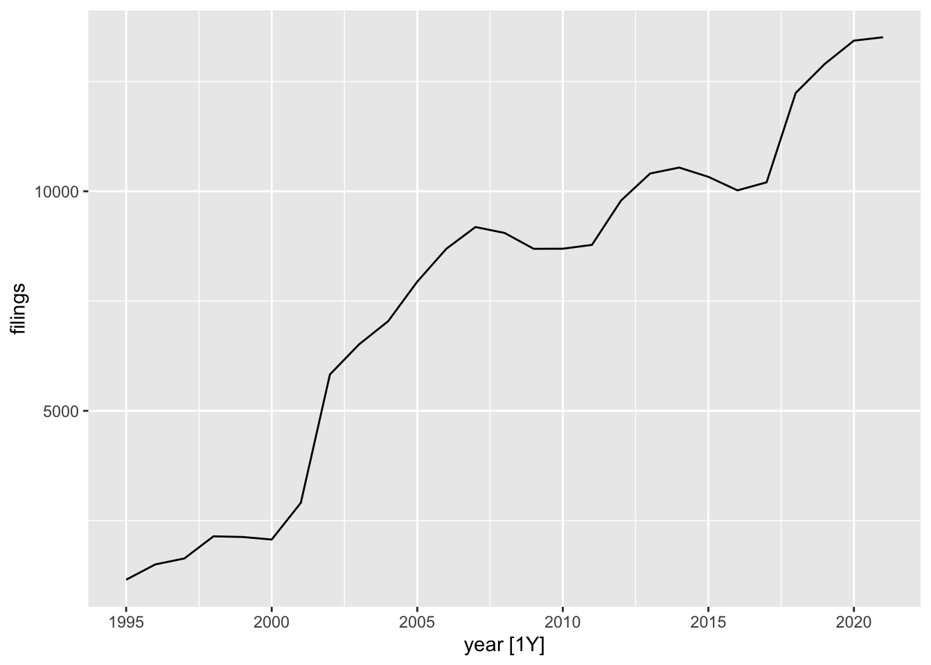

Figure 4.23: PCT Filings with WIPO

Forecasting involves a standard procedure that is illustrated in Figure 4.24 and reproduced from Forecasting: Principles and Practice (3rd ed).

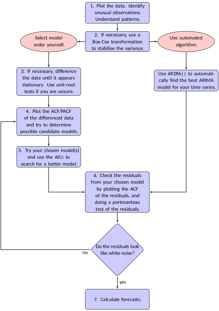
Figure 4.24: Forecasting Procedure

We are presently at step 1: evaluating our data. The key issues to be considered in understanding our time series data are is the data trending (yes) and does it involve seasonality or cyclicity. Seasonality is common in time series data, such as purchasing products at particular times of year. Because our data is yearly it cannot be seasonal.

Cyclicity refers to whether our data is affected by business cycles. This is harder to assess. While the submission of patent applications to the International Bureau is clearly trending upwards, there are some very notable peaks, flat spots and troughs. In the author’s view these are likely to reflect global economic conditions, such as the bursting of the ‘dot com’ bubble in the late 1990s, the financial crisis in 2007-2008 and the stock market crash of 2015-2016. We may be tempted to think of a cycle as a regular predictable series of events. However, in reality cyclicity is represented by irregular events of varying duration.

What we discern from our quick time series plot is that our data is clearly trending and is not seasonal. However, it does display cyclicity and this will be reflected in a skew in the distribution of the data. It is possible to apply various transformations to the data to address this such as the Box-Cox Transformation or differencing to stabilise the data. However, this can rapidly become quite involved and the clock is ticking (see below). We make a mental note to highlight this issue in bold in the presentation of the data.

Using the fable package it is remarkably easy to fit different forecasting models and compare the results with straightforward code. As we are in a rush we will use three models:

1. Naive. The naive model simply takes the last data point and projects it into the future. The naive model therefore assumes that the last observation will continue into the future.

2. ETS is Exponential Smoothing. As Hyndman and Athanasopoulos explain: “Forecasts produced using exponential smoothing methods are weighted averages of past observations, with the weights decaying exponentially as the observations get older.” You can read more about exponential smoothing methods in Chapter 8 of the Forecasting: Principles and Practice (3rd ed)

3. ARIMA stands for Autoregressive Integrated Moving Average and, along with ETS, is one of the most popular sets of forecasting models. The model is autoregressive because it uses past observations to predict the future, and in this case as the name implies, it does this using a lagged moving average.

We start by fitting the models to our data. This is extremely easy to do.

library(tidyverse)
library(fable)


fit <- pct_ts %>%
  model(
    naive = NAIVE(filings),
    ets = ETS(filings),
    arima = ARIMA(filings)
  )
fit

## # A mable: 1 x 3
##     naive          ets                   arima
##   <model>      <model>                 <model>
## 1 <NAIVE> <ETS(A,A,N)> <ARIMA(0,1,0) w/ drift>

After fitting the models we can access a range of statistics with the general aim of identifying the model with the lowest error scores across a range of measures. In particular, when creating several models there are standard measures for comparison that focus on calculation of types error. Of the available measures Hyndman and Athanasopoulos generally recommend the second order AICc (a variant of the Akaike Information Criterion or AIC). Other options include the Bayesian Information Criterion (BIC). We can see below that across three types of information criteria the ARIMA model comes out best (note that some scores are not available for the different models). We can see these scores in Table 4.15.

fit_glance <- fit %>% glance()

fit_glance %>% 
  knitr::kable(caption = "Comparative Model Scores")

Table 4.15: Comparative Model Scores

.model	sigma2	log_lik	AIC	AICc	BIC	MSE	AMSE	MAE	ar_roots	ma_roots
naive	509955.5	NA	NA	NA	NA	NA	NA	NA	NULL	NULL
ets	609713.7	-222.1592	454.3185	457.1756	460.7976	519385.7	1240281	516.8461	NULL	NULL
arima	509955.5	-207.2296	418.4591	418.9809	420.9753	NA	NA	NA

Based on these measures we cad reasonably choose the ARIMA model to present to the DG.

However, before going ahead we realise that we are experiencing an uncomfortable itch from the variance in the data resulting from the financial crises. We can gain an understanding of this itch by inspecting the residuals. Residuals are simply the difference between the observed and predicted values.

The residuals for the ETS model are displayed in Figure 4.25 and for the ARIMA model in Figure 4.26.

library(feasts)
fit %>% select(ets) %>% gg_tsresiduals()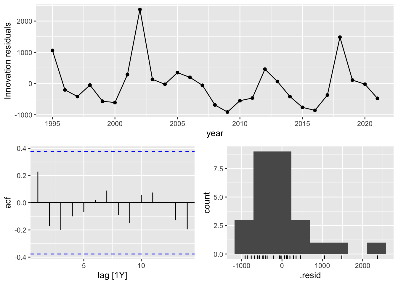

Figure 4.25: Residuals for the ETS fitted model

library(feasts)
fit %>% select(arima) %>% gg_tsresiduals()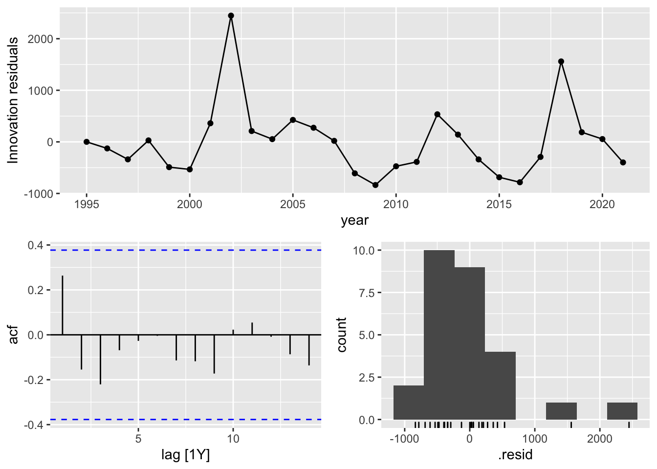

Figure 4.26: Residuals for the ARIMA fitted model

In considering these plots, the residuals are what is left over after a model has been fitted and is made up of the difference between the observed and the fitted values. In assessing the residuals the innovation residuals should not be displaying evidence of a trend. For both models we do not observe evidence of trend although there is clear evidence of significant variance from the mean. The ACF (autocorrelation plot) displays the coefficient of correlation between two values in a time series with a lag of 1. The residuals fall within the boundaries represented by the dotted lines and we are happy enough with the lack of marked outliers in the residuals.

So far, so good. However, the third plot in the residuals report shows the distribution of the data. This should be normally distributed. We can see that our data skews to the left with outliers to the right. The ARIMA model does a better job of distinguishing these outliers.

There are a number of transformations that could be applied to this data to normalise it such as the use of differencing or a Box-Cox Transformation. These can be readily calculated in R using the fable and fabletools packages. However, note that transformations of data can be a subject of controversy.

What are we going to tell the DG? Having inspected our data and being aware that it is rather skewed by cyclic events in the world economy we use our fitted models to produce a forecast.

fc <- fit %>%
  forecast(h = "5 years")

fc %>% 
  head(20) %>% 
  knitr::kable()

.model	year	filings	.mean
naive	2022	N(13508, 716113)	13508.00
naive	2023	N(13508, 1432226)	13508.00
naive	2024	N(13508, 2148339)	13508.00
naive	2025	N(13508, 2864452)	13508.00
naive	2026	N(13508, 3580565)	13508.00
ets	2022	N(14060, 609714)	14059.88
ets	2023	N(14612, 1219427)	14611.72
ets	2024	N(15164, 1829263)	15163.55
ets	2025	N(15715, 2439220)	15715.39
ets	2026	N(16267, 3e+06)	16267.22
arima	2022	N(13983, 509956)	13983.15
arima	2023	N(14458, 1e+06)	14458.31
arima	2024	N(14933, 1529867)	14933.46
arima	2025	N(15409, 2e+06)	15408.62
arima	2026	N(15884, 2549778)	15883.77

Having fitted the model we can plot the three forecasts as in Figure 4.27

fc %>% 
  autoplot(pct_ts)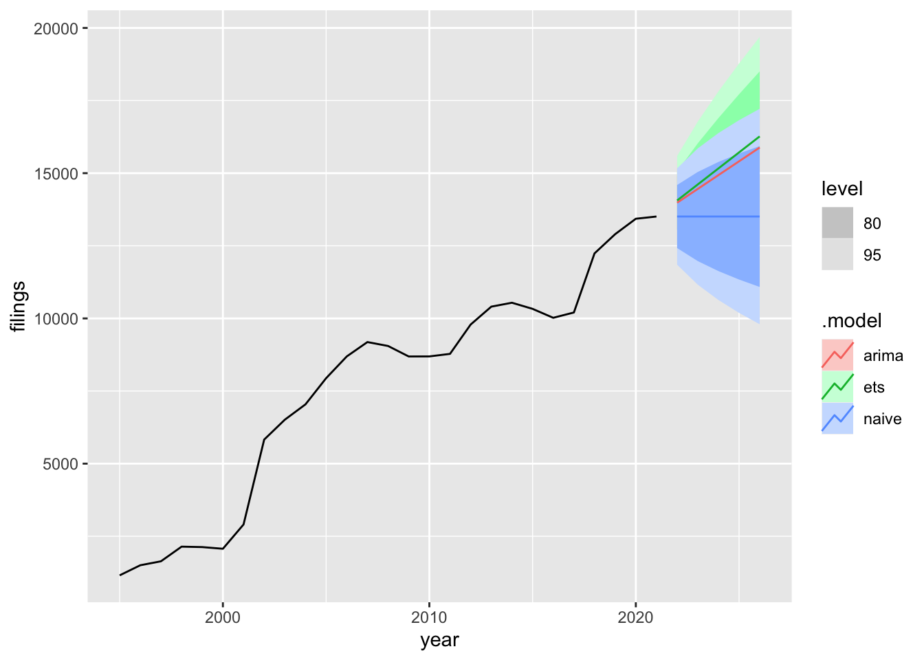

Figure 4.27: Three Forecasts

In interpreting the forecast the three straight lines represent the mean for the forecast produced by each model with the 80% to 95% confidence intervals represented by the corresponding colours. We can clearly see that the ETS model produces the steepest projected forecast with the naive model projecting a straight line from the last data point. Based on the AICc and other scores we will choose the ARIMA model forecast and use the naive model as the as is example.

We can easily drop the ETS model from the figure that we will include in the brief for the DG.

fc %>% 
  filter(.model != "ets") %>% 
  autoplot(pct_ts)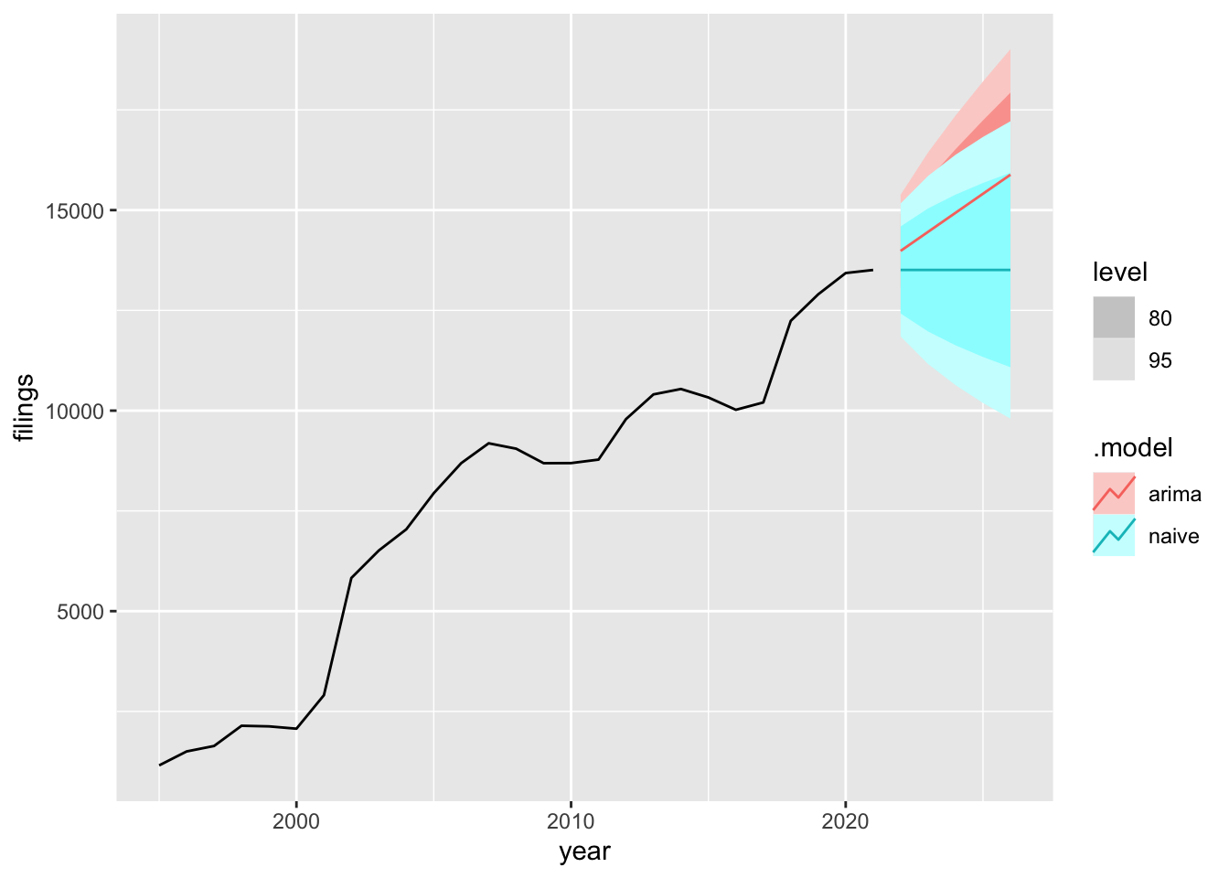

Figure 4.28: As Is and ARIMA Forecasts

The forecasts include the data on the number of projected filings and we can therefore project likely revenue from this data using the rough US$1387 fee value as our assumption.

revenue <- fc %>% 
  filter(.model != "ets") %>% 
  tsibble::tibble() %>% 
  select(.model, year, .mean) 

revenue_asis <- revenue %>% 
  filter(.model == "naive") %>% 
  tsibble::tibble() %>% 
  select(.model, year, .mean) %>% 
  mutate(.mean = round(.mean)) %>% 
  mutate(forecast_revenue_us = .mean * 1387) %>% 
  rename(forecast_filings = .mean) %>% 
  janitor::adorn_totals()

revenue_forecast <- revenue %>% 
  filter(.model == "arima") %>% 
  tsibble::tibble() %>% 
  select(.model, year, .mean) %>% 
  mutate(.mean = round(.mean)) %>% 
  mutate(forecast_revenue_us = .mean * 1387) %>% 
  rename(forecast_filings = .mean) %>% 
  janitor::adorn_totals() 

We can see the results in Table 4.16 and Table 4.17.

Table 4.16: As is Revenue Forecast

.model	year	forecast_filings	forecast_revenue_us
naive	2022	13508	18735596
naive	2023	13508	18735596
naive	2024	13508	18735596
naive	2025	13508	18735596
naive	2026	13508	18735596
Total	10120	67540	93677980

Table 4.17: ARIMA Revenue Forecast

.model	year	forecast_filings	forecast_revenue_us
arima	2022	13983	19394421
arima	2023	14458	20053246
arima	2024	14933	20712071
arima	2025	15409	21372283
arima	2026	15884	22031108
Total	10120	74667	103563129

We will want to write a quick explanation of the models that we have produced and present the forecast numbers. The DG doesn’t like long documents, a page or two at most. We will present the naive model as a forecast for filings and revenue assuming that last years filings continue into the future with no change. This can serve as a useful baseline of what might reasonably be expected. We use the ARIMA model as our actual forecast of filings and revenue which shows a steady upward trend. The difference between total revenue under the ‘as is’ and the ARIMA forecast over the five year period is US$9,885,149. In the note we ensure that we are transparent about the uncertainty created by the skew in the data and recommend that the economists are set to work on it.

There is a knock at the door. It will be the boss. Our two page print out is on the printer. You gulp… pick up the forecast and head off to meet your fate.

Global stock markets crash the next day.

4.10 Conclusion

This chapter has provided a wide ranging practical introduction to patent counts and descriptive patent statistics that concluded with a brief introduction to forecasting. Of all of the chapters in this handbook this is the most important. Arriving at accurate counts of patent data is not straightforward. This chapter has taken you through those issues. We concluded with a brief introduction to linear regression by exploring commonly used linear models and their application to patent data before moving on to exploring ways to generate forecasts and the issues they involve.

In closing it is important to emphasise that there is frequently more than one way to count patent data and the type of count that you use will depend on the question you are seeking to address, the data at hand and what you want to communicate to the audience.

References

Criscuolo, P. 2006. “The ’Home Advantage’ Effect and Patent Families. A Comparison of OECD Triadic Patents, the USPTO and the EPO.” Scientometrics 66: 23–41.

Dechezleprêtre, Antoine, Yann Ménière, and Myra Mohnen. 2017. “International Patent Families: From Application Strategies to Statistical Indicators.” Scientometrics 111 (2): 793–828. https://doi.org/10.1007/s11192-017-2311-4.

Dernis, Hélène. 2007. “Nowcasting Patent Indicators,” January.

Dernis, Hélène, and Mosahid Khan. 2004. “Triadic Patent Families Methodology.” Organisation for Economic Co-Operation; Development (OECD). https://doi.org/10.1787/443844125004.

Hall, Bronwyn H., and Dietmar Harhoff. 2012. “Recent Research on the Economics of Patents.” Annual Review of Economics 4 (1): 541–65. https://doi.org/10.1146/annurev-economics-080511-111008.

Hegde, Deepak, David Mowery, and Stuart Graham. 2007. “Pioneers, Submariners, or Thicket-Builders: Which Firms Use Continuations in Patenting?” National Bureau of Economic Research. https://doi.org/10.3386/w13153.

Lemley, Mark A., and Kimberly A. Moore. 2003. “Ending Abuse of Patent Continuations.” SSRN Electronic Journal. https://doi.org/10.2139/ssrn.462404.

Martinez, Catalina. 2010a. “Insight into Different Types of Patent Families.” Organisation for Economic Co-Operation; Development (OECD). https://doi.org/10.1787/5kml97dr6ptl-en.

———. 2010b. “Patent Families: When Do Different Definitions Really Matter?” Scientometrics 86 (1): 39–63. https://doi.org/10.1007/s11192-010-0251-3.

OECD Patent Statistics Manual. 2009. OECD Publishing. https://doi.org/10.1787/9789264056442-en.

Sternitzke, Christian. 2009. “Defining Triadic Patent Families as a Measure of Technological Strength.” Scientometrics 81 (1): 91–109. https://doi.org/10.1007/s11192-009-1836-6.

Wickham, Hadley. 2022. Modelr: Modelling Functions That Work with the Pipe.

---

8. WIPO Summary of the Paris Convention for the Protection of Industrial Property (1883) http://www.wipo.int/treaties/en/ip/paris/summary_paris.html↩︎

9. The observant reader will note that for reasons that are entirely unclear publication of the granted patent in 2016 takes place before the publication of the application in 2017↩︎

10. Counts were cross validated in Vantage Point in light of the spike in B publications between 2000 and 2001↩︎

11. This topic was discussed a number of years ago on the EPO PATSTAT forum but may not have been formally written up.↩︎

12. Martinez notes that PATSTAT data from the 2008 edition may vary in subsequent editions, for example new documents may be added that increase the size or new data sources may be included in PATSTAT↩︎

13. This example can be identified in esp@cenet with application number JP200944799A https://worldwide.espacenet.com/publicationDetails/biblio?FT=D&date=20090820&DB=EPODOC&locale=en_EP&CC=JP&NR=2009184358A&KC=A&ND=4↩︎

14. https://www.print21.com.au/news/kia-silverbrook-dumps-name-as-business-gets-thrashed↩︎

15. Thirty priorities are associated with this patent family. There are two documents that share the earliest date AU19977991A 1997-07-15 and AU19978004A 1997-07-15. esp@cenet lists the earliest priority as AU1997PO08010 19970715. The use of the letter P suggests that this could be some form of provisional filing although we have not been able to trace the use of this kind code in WIPO’s examples for Australia.↩︎

16. esp@cenet Legal Status for US9584681B2↩︎