Chapter 7 Text Mining
Text mining involves the extraction of information from text sources. In the case of the scientific literature and patent data, text mining is closely associated with the concept of technology or tech mining as popularised by Alan Porter and Scott Cunningham (Porter and Cunningham 2004). However, the rise and rise of social media has expanded text mining into the pursuit of insights from platforms Twitter and other social media platforms involving topic modelling and sentiment analysis to inform decision making on public perceptions of technology and responses to products. A dynamic Lens collection on text mining has been created to complement this chapter and will allow you to explore the diverse uses of text mining.
What we might call classic approaches to text mining are rapidly being blended with or replaced by machine learning approaches to Natural Language Processing. We consider machine learning based approaches in the next chapter. In this chapter we focus on some of the basics of text mining and argue that rather than jumping into machine learning based approaches a great deal can be achieved using standard text mining approaches. Standard approaches to text mining have the advantage that they are relatively straightforward to implement and are transparent to the analyst. This is not always true for machine learning based approaches. Perhaps more importantly, an understanding of standard text mining techniques provides a platform for engaging with machine learning based approaches considered in the next chapter.
To introduce text mining we will use the popular tidytext approach using R. This differs from the classic use of a corpus of texts and the creation of document terms matrices that you might have come across elsewhere. An major advantage of the tidytext approach is that the data is easy to understand, visualise and keep track of during transformation steps. In particular, it is easy to retain the document identifiers that are the key to joining to patent text data with other patent data.
This chapter draws heavily on and reproduces code examples from Text Mining with R: A Tidy Approach by Julia Silge and David Robinson. This book is strongly recommended for anyone seeking to engage in text mining and is available free of charge at https://www.tidytextmining.com/. We will use code examples from Text Mining with R to illustrate different approaches. However, we will use a large dataset of texts from US PatentsView service in the worked examples. We will also demonstrate how the International Patent Classification allows us to focus our text mining efforts in relevant areas of the patent system.
The examples in this chapter are designed to illustrate tidy text mining at the scale of millions of records. If the worked examples prove challenging on your computer we recommend that you reduce the size of the examples. The examples in Text Mining with R using the texts of Jane Austen and other classic literature are also highly accessible for working at a smaller scale.
7.1 The USPTO Patent Granted Data
In the last chapter on patent classification we used the ipcr table from the US PatentsView Service to explore uses of the International Patent Classification. In this chapter we will use the patents table for patents granted in the United States. At the time of writing that table consists of 7.8 million documents with the patents table containing identifier information, the titles and the abstracts. You can download the latest version of this table to your machine from the following address.
"https://s3.amazonaws.com/data.patentsview.org/download/patent.tsv.zip" Building on the discussion in the last chapter on patent classification we will also download the latest version of the ipcr table that is available from here.
"https://s3.amazonaws.com/data.patentsview.org/download/ipcr.tsv.zip" One issue with .zip files is that they may not always read in correctly without being unzipped first. Unzip the files on your machine either using a built in application or programatically. We then read in the file. We will be using R and the tidytext package but it is straightforward to read in this data in Python with Pandas.
We will read in a selection of the columns that we will use. To assist with joining our tables we will rename the id column in the grants table as this is called patent_id in the ipc table. We will also create a publication number by joining up the country, number and kind columns. That can assist us with looking up documents online or preparing data for joining to other databases (such as PATSTAT). We can also vary the separator e.g. use “_” depending on the format used by the external database. Table 7.1 displays a selection of the data.
library(tidyverse)
library(vroom)
grants <- vroom::vroom("data/text_mining/patent.csv.gz", show_col_types = FALSE) %>%
  select(id, country, number, kind, title, abstract, date) %>%
  rename(patent_id = id) %>%
  mutate(year = lubridate::year(date)) %>%
unite(publication_number, c(country, number, kind), sep = "", remove = TRUE)| patent_id | publication_number | title |
|---|---|---|
| 10000000 | US10000000B2 | Coherent LADAR using intra-pixel quadrature detection |
| 10000001 | US10000001B2 | Injection molding machine and mold thickness control method |
| 10000002 | US10000002B2 | Method for manufacturing polymer film and co-extruded film |
| 10000003 | US10000003B2 | Method for producing a container from a thermoplastic |
| 10000004 | US10000004B2 | Process of obtaining a double-oriented film, co-extruded, and of low thickness made by a three bubble process that at the time of being thermoformed provides a uniform thickness in the produced tray |
In the previous chapter we worked with the PatentsView IPC table. The raw table contains a ‘patent_id’ field that we can link with other tables and a set of columns with different ipc levels that we can use to construct the four character subclass (e.g. C12N) with. We will use this table below with the patent_id field as the basis for joining with the titles and abstracts. Table 7.2 shows a sample of patent ids and IPC subclass from the cleaned ipcr field. This code also illustrates the use of the dplyr::case_when() function to correct missing zeros in IPC classes in the raw ipcr table as an alternative to the use of if statements.
ipcr <- vroom::vroom("data/text_mining/ipcr.csv.gz", show_col_types = FALSE) %>%
  mutate(ipc_class =
           case_when(

             nchar(ipc_class) == 1 ~ paste0(0,ipc_class),
             nchar(ipc_class) > 1 ~ ipc_class

                       )
           ) %>%
  unite(ipc_subclass, c(section, ipc_class, subclass), sep = "", remove = FALSE) %>%
  select(patent_id, ipc_subclass) %>%
mutate(ipc_subclass = str_to_upper(ipc_subclass))| patent_id | ipc_subclass |
|---|---|
| 6864832 | G01S |
| 9954111 | H01L |
| 10048897 | G06F |
| 10694566 | H04W |
| D409748 | D2404 |
| 7645556 | G03F |
| 8524174 | B01L |
| 10008744 | H01M |
| 11046328 | B60W |
| 9508104 | G06Q |
7.2 Words
A primary task in text mining is tokenizing. A token is a unit in a text, typically a word or punctuation. Phrases are formed from combinations of tokens and sentences are formed from a set of tokens with marker (a full stop) at the end of the sentence. Tokenizing is therefore the process of breaking down texts into their constituent tokens (elements). Tokenizing normally focuses on words (unigrams), phrases (bigrams or trigrams) but extends to sentences and paragraphs.
The tidytext package has a function called unnest_tokens() that by default will tokenize words in a text and will also remove punctuation and turn the case to lowercase. The effect of converting to lowercase is that words such as drone, Drone or DRONE will all be converted to the same case (drone) making for more accurate groupings and counts. Removing punctuation limits the amount of pointless characters in our results.
What is important about tidytext is that it preserves the patent_id as the identifier for each word. This means that we know which document each individual word appears in. This makes it very powerful for dictionary based matches of patent documents. To illustrate, we create a table called grant_words. Depending on how much memory you have this should take a few minutes to run. By default the tidytext package will convert the text to lowercase and remove punctuation. Converting to lowercase makes counts accurate and removing punctuation removes text elements that are not useful for most tasks. Note that you will not always want to convert text to lowercase.
library(tidytext)

grant_words <- grants %>%
  select(patent_id, publication_number, title) %>%
  unnest_tokens(word, title)
When we have processed the text we will see that out 7.9 million individual document titles have expanded to 60,839,863 rows containing words in documents as we see in Table 7.3 which shows words appearing in the titles per document. The important point here is that we know exactly what words appear in each patent document which is a very powerful tool.
| patent_id | publication_number | word |
|---|---|---|
| 10000000 | US10000000B2 | coherent |
| 10000000 | US10000000B2 | ladar |
| 10000000 | US10000000B2 | using |
| 10000000 | US10000000B2 | intra |
| 10000000 | US10000000B2 | pixel |
| 10000000 | US10000000B2 | quadrature |
| 10000000 | US10000000B2 | detection |
| 10000001 | US10000001B2 | injection |
| 10000001 | US10000001B2 | molding |
| 10000001 | US10000001B2 | machine |
| 10000001 | US10000001B2 | and |
| 10000001 | US10000001B2 | mold |
| 10000001 | US10000001B2 | thickness |
| 10000001 | US10000001B2 | control |
| 10000001 | US10000001B2 | method |
| 10000002 | US10000002B2 | method |
| 10000002 | US10000002B2 | for |
| 10000002 | US10000002B2 | manufacturing |
| 10000002 | US10000002B2 | polymer |
| 10000002 | US10000002B2 | film |
As this makes clear, it is very easy to break a document down into its constituent words with tidytext.
7.3 Removing Stop Words
As we can see in Table 7.3 there are many common words such as “and” that do not contain useful information. We can see the impact of these terms if we count up the words as we see in Table 7.4.
| word | n |
|---|---|
| and | 3266729 |
| for | 2974726 |
| method | 1859165 |
| of | 1732262 |
| a | 1499277 |
| system | 1014262 |
| device | 997272 |
| apparatus | 978236 |
| with | 739534 |
| the | 651349 |
| in | 588004 |
| methods | 366751 |
| an | 340798 |
| to | 336512 |
| same | 300901 |
| using | 300292 |
| control | 294340 |
| having | 271477 |
| process | 244300 |
| image | 232694 |
In Table 7.4 we can see that common words will rise to the top but do not convey useful information. For this reason a common approach in text mining is to remove so called ‘stop words’. Exactly what counts a stop word may vary depending on the task at hand. However, certain words such as a, and, the, for, with and so on are not useful if we want to understand what a text or set of texts is about.
In tidytext there is a built in table of stop words and lists of stop words can be found on the internet that you can readily edit to meet your needs. We can see some of the stop words from tidytext in Table 7.5. In reality tidytext includes three lexicons of stop words (onix, SMART and snowball) that you can use or adapt for your needs. There are also options to add your own.
| word | lexicon |
|---|---|
| a | SMART |
| a’s | SMART |
| able | SMART |
| about | SMART |
| above | SMART |
| according | SMART |
| accordingly | SMART |
| across | SMART |
| actually | SMART |
| after | SMART |
Applying stop words to our grant titles is straightforward. In the code below we first create a new column that matches words in the stopword list. We then filter them out (the same code can be written in various ways).
grant_words_clean <- grant_words %>%
  select(patent_id, word) %>%
  mutate(stop = word %in% tidytext::stop_words$word) %>%
  filter(stop == FALSE)
This reduces our 60.8 million row dataset to 44 million, losing nearly 17 million words.
Now when we count up the words in the grants titles we should get some more useful results as we see in Table 7.6.
| word | n |
|---|---|
| method | 1859165 |
| system | 1014262 |
| device | 997272 |
| apparatus | 978236 |
| methods | 366751 |
| control | 294340 |
| process | 244300 |
| image | 232694 |
| data | 232002 |
| display | 218565 |
| systems | 201809 |
| circuit | 192200 |
| semiconductor | 187196 |
| thereof | 184853 |
| processing | 184550 |
| vehicle | 175908 |
| assembly | 174347 |
| manufacturing | 172285 |
| power | 163450 |
| optical | 156712 |
We can make two observations about Table 7.6. The first of these is that there are some words that appear quite commonly in patents such as “thereof” that we would want to add to our own stop words list (others might be words like comprising). However, we would want to take care with other potential stop words that may provide us with information about the type of patent claims (such as composition for composition of matter, methods and process) that we would probably want to keep for some purposes (for example if examining patent claims).
7.4 Lemmatizing words
The second observation is that there are pluralised forms of some words, such as method, methods, process, processing, processes and so on. These are words that can be grouped together based on a shared form (normally the singular such as method and process). These groupings are known as lemmas. It is important to emphasise that lemmatizing is distinct from stemming words, which reduces words to a common stem.
There are a variety of tools out there for lemmatizing text. We will use the textstem package by Tyler Rinker (Rinker 2018) in R which provides a range of options for lemmatizing words. In the code below we will create a new column with the lemmatized version of words called lemma. We will filter out any digits at the same time. Here we lemmatize the words that we have already applied stop words to.
library(textstem)

grant_lemma <- grant_words_clean %>%
  mutate(word = str_trim(word, side = "both")) %>%
  mutate(lemma = lemmatize_words(word)) %>%
  mutate(digit = str_detect(word, "[[:digit:]]")) %>%
  filter(digit == FALSE) %>%
  select(-digit)
If we count up our lemmatized words we will see a dramatic change in the scores for terms such as ‘method’ and ‘process’ as we see in Table 7.7.
| lemma | n |
|---|---|
| method | 2225916 |
| system | 1216071 |
| device | 1122573 |
| apparatus | 991158 |
| process | 451231 |
| control | 420688 |
It is important to be cautious with lemmatizing to ensure that you will be getting what you expect. However, it is a particularly powerful tool for harmonising data to enable aggregation for counts. As we will also see, this is an important for topic modelling and network visualization.
We now have a clearer idea of the top terms that appear across the corpus of US patent grants. As we will see below, if we know what words we are interested in we could simply identify all of the documents that contain those words for further analysis.
As discussed in the discussion of the patent landscape for animal genetic resources in the last chapter on classification, the use of a dictionary of terms such as pig, horse, cow and so on allows us to capture a universe of documents that contain animal related terms. However, this will also catch a lot of extraneous noise from uses of terms that are difficult for the analyst to predict in advance (such as pipeline pigs and clothes horses).
What is important in the case of the patent system is that we can leverage the patent classification to help us refine our text mining efforts.
To illustrate this we will start by using a well known measure known as “term frequency inverse document frequency” (TFIDF) to understand what terms are distinctive in our set for particular areas of technology.
7.5 Terms by Technology
As an experiment we will see what the terms are in four areas of technology using IPC subclasses. For this experiment, we will use examples that are distinctive and some that are likely to overlap, these are:
- Plant agriculture (A01H),
- Medicines and pharmaceuticals (A61K),
- Biotechnology (C12N)
- Computing (G06F)
To do this we will start by identifying the patent_ids that fall into these subclasses with the results shown in Table 7.8.
ipc_set <- ipcr %>%
  select(patent_id, ipc_subclass) %>%
  filter(., ipc_subclass == "A01H" | ipc_subclass == "A61K" |
ipc_subclass == "C12N" | ipc_subclass == "G06F")| patent_id | ipc_subclass |
|---|---|
| 10048897 | G06F |
| PP10471 | A01H |
| 9600201 | G06F |
| 9138474 | A61K |
| 9898174 | G06F |
| 9836588 | G06F |
This gives us a total of just over 2.4 million patent_ids that have one or more of these classifiers.
We now join the two tables by the patent_id using inner_join. In SQL (here written with dplyr in R) an inner join is a filtering join that will keep only shared elements in the two tables (the patent_ids). We then count the words and sort them as we see in Table 7.9.
ipc_words <- ipc_set %>%
  inner_join(grant_lemma, by = "patent_id") %>%
count(ipc_subclass, lemma, sort = TRUE)| ipc_subclass | lemma | n |
|---|---|---|
| G06F | method | 597874 |
| G06F | system | 507874 |
| G06F | device | 252371 |
| G06F | datum | 210127 |
| G06F | apparatus | 205122 |
| A61K | method | 190228 |
For the calculation that we are about to make using the code provided by Silge and Robinson we first need to generate a count of the total number of words for each of our technology areas (subclasses). To do that we group the table by ‘ipc_subclass’ so that we can count up the words in each subclass (rather than the whole table). It is important to ungroup() the data at the end. The reason for this is that without ungrouping any future operations such as counts will be performed on the grouped table leading to unexpected results and considerable confusion.
ipc_total_words <- ipc_words %>%
  group_by(ipc_subclass) %>%
  summarise(total = sum(n)) %>%
  ungroup()
Next we join the two tables together using left_join(). Unlike inner_join(), left_join() will keep everything in our original ipc_words table on the left hand side (that we will be applying the TFIDF to).
ipc_words <- ipc_words %>%
  left_join(ipc_total_words, by = "ipc_subclass")
We are now in a position to apply the term frequency inverse document frequency calculations (using bind_tf_idf) as we see in Table 7.10.
library(tidytext)
ipc_words_tfid <- ipc_words %>%
  bind_tf_idf(word, ipc_subclass, n) %>%
  arrange(desc(tf_idf))

ipc_words_tfid| ipc_subclass | word | n | tf | idf | tf_idf |
|---|---|---|---|---|---|
| A01H | inbred | 5275 | 0.0149659 | 0.6931472 | 0.0103735 |
| A01H | cultivar | 7995 | 0.0226828 | 0.2876821 | 0.0065254 |
| A01H | rose | 3421 | 0.0097058 | 0.2876821 | 0.0027922 |
| A01H | calibrachoa | 641 | 0.0018186 | 1.3862944 | 0.0025211 |
| A01H | hydrangea | 584 | 0.0016569 | 1.3862944 | 0.0022969 |
| G06F | server | 22500 | 0.0016522 | 1.3862944 | 0.0022905 |
The application of the bind_tf_idf function gives us a term frequency score (tf) an inverse document frequency score (idf) and a term frequency inverse document frequency score as a product of term frequency and inverse document frequency. In straightforward terms, this gives us a calculation of how distinctive a particular term is in the set of words within a document or group of documents.
We can visualise the distinctive terms from the titles of publications for the four distinctive subclasses in Figure 7.1.
ipc_names <- c(
  'A01H'="Plant Agriculture (A01H)",
  'C12N'="Biotechnology (C12N)",
  'A61K'="Pharmaceuticals (A61K)",
  'G06F'="Computing (G06F)"
)

ipc_words_tfid %>%
  arrange(desc(tf_idf)) %>%
  mutate(word = factor(word, levels = rev(unique(word)))) %>%
  group_by(ipc_subclass) %>%
  top_n(15) %>%
  ungroup() %>%
  ggplot(aes(word, tf_idf, fill = ipc_subclass)) +
  geom_col(show.legend = FALSE) +
  labs(x = NULL, y = "tf_idf") +
  facet_wrap(ipc_subclass ~., labeller = as_labeller(ipc_names), ncol = 2,
             scales = "free") +
  coord_flip()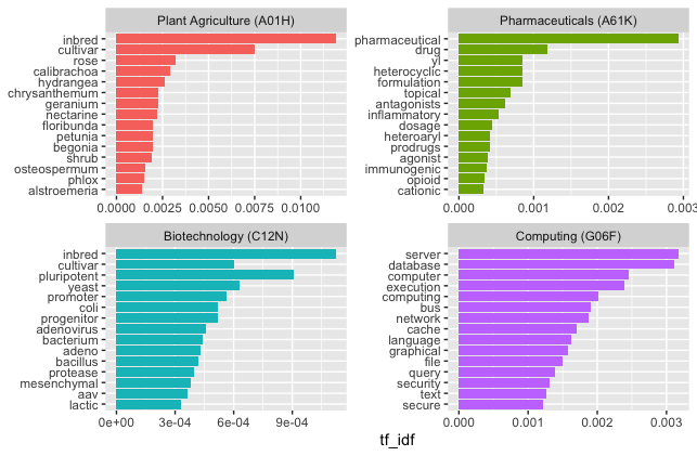
Figure 7.1: TFIDF scores for distinctive terms in patent titles by IPC subclass
In the original example that we are copying here from Silge and Robinson, the different novels written by Jane Austen were mainly distinguished not by the language used but by the names (proper nouns) of the individual characters in each novel, such as Darcy in Pride and Prejudice and Emma and Knightley in Emma. In contrast, when ranked by tfidf our patent data displays very distinctive terms associated with each subclass, with some overlap between A01H and C12N. In the case of plant agriculture and biotechnology this will arise from genetically modified plants (which fall into both categories of the system), Note that in the case of A61K we appear to have some partial words (e.g. yl) arising from the process of splitting the text into tokens. A solution here would be to filter out words with 2 or 3 characters or less unless there is a good reason not to. This example quite vividly illustrates the point that term frequency inverse document frequency, and its multiple variants in use by search engines, is a very powerful means of picking out distinctive terms in groups of documents and for modelling the topics that these documents are about. However, these examples also illustrate the importance of the patent classification.
7.6 Combining Text Mining with Patent Classification
In reality, the distinctive terms that we observe in Figure 7.1 reinforce the point made in the last chapter: the patent classification is our friend. In contrast with many other forms of document systems the patent system uses a sophisticated human and machine curated international classification system to describe the content of patent documents. The importance of engaging with the classification to assist with text mining is revealed by the terms in the different subclasses: the classification does a lot of work for us. Once we understand the classification we are able to target our attention to areas of the system that we are interested in. Put another way, rather than starting by text mining the titles or other text elements of all patent documents we will save ourselves a lot of time and effort by targeting our efforts to specific areas of the system using the international patent classification as our guide.
We can briefly illustrate this point using the topic of drones using the patent titles.
grant_lemma %>%
  filter(lemma == "drone") %>%
  inner_join(ipcr, by = "patent_id") %>%
count(ipc_subclass, sort = TRUE)| ipc_subclass | n |
|---|---|
| B64C | 816 |
| G05D | 567 |
| B64D | 368 |
| H04W | 368 |
| G08G | 319 |
| G01S | 267 |
In practice, we would want to use larger text segments such as titles and abstracts rather than simply the titles (see below). However, this example illustrates that if we wanted to start exploring the topic of drone technology we would probably want to include B64C (Aeroplanes and Helicopters), G05D (control systems) and B64D (aircraft equipment) as part of our search strategy for the straightforward reason that these are areas of the patent library where documents containing these words are to be found.
We can scale up this example to focus on a broader topic area of wider policy interest: biodiversity. In previous work, Oldham, Hall and Forero text mined the full text of 11 million patent documents for millions of taxonomic species names using regular expressions (P. Oldham, Hall, and Forero 2013). This research also revealed that it is possible to capture the majority of biodiversity related terms by focusing on specific areas of the patent classification. Use of a set of English terms within those areas of the system would then capture the universe of documents that need to be captured. The two elements of that search strategy involved a set of terms that commonly appear in biodiversity related documents and a set of IPC classes.
The search terms are presented below. As these are search terms that are designed to be used in a search engine they include plurals and are not stemmed to avoid capturing many irrelevant terms.
biodiversity_ipc_words <- tibble(word = c("species","genus","family","order","phylum","class","kingdom","tribe","dna",
  "nucleic","nucleotide","amino","polypeptide","sequence","seq","seqid", "protein",
  "proteins","peptides","peptide","enzyme","enzymes","plant","plants","animal","animals","mammal",
  "mammals","mammalian","bacteria","bacterium","protozoa","virus","viruses","fungi","animalia","archaea",
  "chromista","chromist","chromists","protista","protist","protists","plantae","eukarya","eukaryotes",
  "eukaryote","prokarya","prokaryote","prokaryotes","microorganism","microorganisms","organism","organisms",
  "cell","cells","gene","genes","genetic","viral","biological","biology","strain","strains","variety","varieties",
  "accession"))
For this example we will scale up to include words from both the titles and abstracts of US granted patents. We will do this by uniting the titles and the abstracts into one string and then breaking that into words. Note that this is RAM intensive and if working on a machine with limited RAM you may wish to filter the grants data to a specific year to try this out. As an alternative, it is now very cost effective to create a powerful virtual machine with a cloud computing service (Amazon Web Services, Google Cloud, Microsoft Azure etc.) that can be destroyed when a task is completed. The use of cloud computing is beyond the scope of this Handbook but is extremely useful for working with data at scale using either VantagePoint (on Windows Server) or with programming languages such as R, Python, Spark or Google Big Query. Many guides to getting started with creating virtual machines are available online and packages exist in R and Python that allow you to create and manage virtual machines from your desktop. Other options include Remote Desktop (for accessing remote virtual Windows machines as if they are your local desktop). We start by restricting the data to the identifier and title and abstract which we combine together before splitting into words. We then remove stop words. For this illustration we will not perform additional clean up steps.
words_ta <- grants %>%
  select(patent_id, title, abstract) %>%
  unite(text, c(title, abstract), sep = ". ") %>%
  unnest_tokens(word, text)  %>%
  mutate(stop = word %in% tidytext::stop_words$word) %>%
  filter(stop == FALSE) %>%
select(-stop)| patent_id | word |
|---|---|
| 10000000 | coherent |
| 10000000 | ladar |
| 10000000 | intra |
| 10000000 | pixel |
| 10000000 | quadrature |
| 10000000 | detection |
This gives us a raw dataset with 893,067,757 rows that reduces to 475,833,395 when stop words are removed. We now match our cleaned up terms to our biodiversity dictionary.
We now want to reduce the set to those documents that contain our biodiversity dictionary. With this version of the US grants table we obtain a ‘raw hits’ dataset with 2,692,948 rows and 805,675 raw patent grant documents. In the second step we want to join to the IPC to see what the top subclasses are. We combine these steps in the code below. We use inner_join to filter the documents to those containing the biodiversity terms and left_join for the IPC.
biodiversity_words <- words_ta %>%
  inner_join(biodiversity_ipc_words, by = "word") %>%
  left_join(ipcr, by = "patent_id")
This will produce a dataset with our biodiversity terms and 2084 IPC subclasses. Table 7.11 shows the top 20 subclasses.
| ipc_subclass | n |
|---|---|
| C12N | 1151393 |
| A61K | 1034746 |
| A01H | 590274 |
| C07K | 514985 |
| H01M | 348670 |
| G01N | 344056 |
| H01L | 323959 |
| G11C | 309924 |
| C12Q | 288365 |
| H04W | 259230 |
| G06F | 247670 |
| C12P | 245579 |
| C07H | 220449 |
| C07D | 175588 |
| H04L | 136105 |
| A01N | 134383 |
| H04N | 80492 |
| A61B | 76849 |
| C07C | 64242 |
| H04B | 55282 |
A total of 1,773 IPC subclasses include our biodiversity terms. In considering Table 7.11 we can make three key observations. The first of these is that we have a clear concentration of the biodiversity related terms in certain areas of the patent system. The second observation is that this data includes subclasses in section G and H of the classification that are very unlikely to have anything to do with biodiversity as such. For example, words in our set such as ‘order’ for the taxonomic rank are likely to create a lot of noise from systems that involve ordering in all its various forms (and should perhaps be removed). The third observation is that we can safely exclude areas that are likely to constitute noise by classification.
One feature of the patent system is that documents receive multiple classification codes to describe the contents of a document. Excluding subclasses such as G01N will only have the effect of excluding documents that don’t contain one of the other ‘keep’ classifiers. That is, documents classified as both C12N and GO1N will be retained because of the presence of C12N. Drawing on this logic we can arrive at a set of subclasses that can be used as a filter for the biodiversity terms and constitute core classifiers for biodiversity. Note that in one case (subclass C02F) we would confine a search engine based search to C02F3 (for biological treatments of waste water and sewage) as the only relevant group in the subclass.
biodiversity_ipc_subclass <- tibble(
  ipc_subclass = c("A01H","A01K","A01N","A23L","A23K","A23G","A23C","A61K","A61Q",
                   "C02F","C07C","C07D","C07H","C07K","C08H","C08L","C09B","C09D",
                   "C09G","C09J","CO9K","C11B","C11C","C11D","C12M","C12N","C12P",
                   "C12Q","C12R","C12S","C40B"))
At present we have a set of biodiversity words. What we want to do next is to filter the documents to the records that contain a biodiversity word AND appear in one of the subclasses above. We then want to count up the patent_ids and obtain the grants (containing the titles, abstracts and other information) for further analysis. We achieve this by first filtering the data to those containing the subclasses, then we count the patent identifiers to create a distinct set and join on to the main patent grants table using the patent ids. Table 7.12 shows the outcome of joining the data back together again.
| patent_id | publication_number | title |
|---|---|---|
| 10000393 | US10000393B2 | Enhancement of dewatering using soy flour or soy protein |
| 10000397 | US10000397B2 | Multiple attached growth reactor system |
| 10000427 | US10000427B2 | Phosphate solubilizing rhizobacteria bacillus firmus as biofertilizer to increase canola yield |
| 10000443 | US10000443B2 | Compositions and methods for glucose transport inhibition |
| 10000444 | US10000444B2 | Fluorine-containing ether monocarboxylic acid aminoalkyl ester and a method for producing the same |
| 10000446 | US10000446B2 | Amino photo-reactive binder |
At the end of this process we have 345,975 patent grants that can used for further analysis using text mining techniques. Our purpose here has been to illustrate how the use of text mining can be combined with the use of the patent classification to create a dataset that is much more targeted and a lot easier to work with. Put another way, it is a mistake to see the patent system as a giant set of texts that all need to be processed. It is better to approach the patent system as as a collection of texts that have already been subject to multi-label classification. That classification can be used to filter to collections of texts for further analysis.
More advanced approaches to those suggested here for refining the texts to be searched, such as the use of matrices and network analysis were discussed in the previous chapter and we return to this topic below. Other options include selecting texts on the IPC group or subgroup level (bearing in mind that for international research not all patent offices will consistently use these levels). The key point here however is that we have moved from a starting set of 7.9 million patent documents and reduced the set to 338,837 documents that are closer to a target subject area. In the process we have reduced the amount of compute effort required for analysis and also the intellectual effort required to handle such large volumes of text.
7.7 From words to phrases (ngrams)
We have focused so far on text mining using individual word tokens (unigrams). However, in many cases what we are looking for will be expressed in a phrase consisting of two (bigram) or three (trigram) strings of words that articulate concepts or are the names of entities (e.g. species names).
The tidytext package makes it easy to tokenize texts into bigrams or trigrams by specifying an argument to the unnest_tokens() function or using the unnest_ngrams() function. We will focus here on bigrams. Note that for chemical compounds which often consist of strings of terms linked by hyphens, attention would need to be paid to adjusting the tokenisation to avoid splitting on hyphens.
biodiversity_texts <- biodiversity_patent_ids %>%
  unite(text, c(title, abstract), sep = ". ")
Table 7.13 shows a selection of the bigrams appearing in the biodiversity related texts.
| patent_id | n | publication_number | bigram |
|---|---|---|---|
| 10000393 | 12 | US10000393B2 | enhancement of |
| 10000393 | 12 | US10000393B2 | of dewatering |
| 10000393 | 12 | US10000393B2 | dewatering using |
| 10000393 | 12 | US10000393B2 | using soy |
| 10000393 | 12 | US10000393B2 | soy flour |
| 10000393 | 12 | US10000393B2 | flour or |
We have created a dataset of bigrams that contains 31,612,494 rows with a few lines of code. However, if we inspect the bigrams we will see that the data contains phrases including many stop words. In reality, in patent analysis we are almost always interested in nouns, proper nouns and noun phrases.
To get closer to what we want, Silge and Robinson present a straightforward approach to removing stop words that involves three steps:
- splitting the bigrams into two columns containing unigrams using the space as the separator
- Filtering out stop words in the two columns
- Combining the two columns back together again.
These steps comply with a common analysis pattern called split - apply - combine. In this case we split up the texts, then apply a function to transform the data and recombine. Becoming familiar with this basic formula is helpful in thinking about the steps involved in text mining and in data analysis in general. Depending on the size of the dataset this will take some time to run because it iterates over word one and word two columns identifying stop words in each row.
clean_biodiversity_bigrams <- biodiversity_bigrams %>%
  separate(bigram, into = c("one", "two"), sep = " ") %>%
  filter(!one %in% tidytext::stop_words$word) %>%
  filter(!two %in% tidytext::stop_words$word) %>%
  unite(bigram, c(one, two), sep = " ")
As before this will radically reduce the size of the dataset to 9,321,285 although the set may still contain many irrelevant phrases as we can see in Table 7.14.
| patent_id | n | publication_number | bigram |
|---|---|---|---|
| 10000393 | 12 | US10000393B2 | soy flour |
| 10000393 | 12 | US10000393B2 | soy protein |
| 10000393 | 12 | US10000393B2 | protein dewatering |
| 10000393 | 12 | US10000393B2 | dewatering agents |
| 10000393 | 12 | US10000393B2 | dewatering wastewater |
| 10000393 | 12 | US10000393B2 | wastewater slurries |
We now have a set of bigrams with many irrelevant phrases. We could simply filter these phrases for terms of interest. In the chapter on patent citation analysis we focus on genome editing technology which is closely linked to genome engineering and synthetic biology. The extraction of bigrams allows us to identify patent grants containing these terms of interest in the title or abstracts as we can see in the code below and Table 7.15.
clean_biodiversity_bigrams %>%
  filter(bigram == "genome editing" | bigram == "gene editing" | bigram == "crispr cas9" |
           bigram == "synthetic biology" | bigram == "genome engineering") %>%
count(bigram)| patent_id | n | publication_number | bigram |
|---|---|---|---|
| 10000800 | 4 | US10000800B2 | synthetic biology |
| 10006054 | 12 | US10006054B1 | genome editing |
| 10011850 | 12 | US10011850B2 | genome editing |
| 10011850 | 12 | US10011850B2 | genome editing |
| 10017825 | 12 | US10017825B2 | genome editing |
| 10047355 | 54 | US10047355B2 | gene editing |
This is a powerful technique for identifying useful documents based on dictionaries of terms (bigrams or unigrams). At an exploratory stage it also be very useful to arrange a bigrams set alphabetically so that you can see what terms are in the immediate vicinity of a target term. This can pick up variants that will improve data capture and links to correlations between terms discussed below.
However, we are still dealing with 9.5 million terms. Can we make this more manageable? The answer is yes. We can apply the tf_idf calculations we used for unigrams above to the bigrams. In this case we are applying the tf_idf calculation to the 345,975 patent grants in the biodiversity set (rather than IPC subclasses) to ask the question: What bigrams are distinctive to each document? As with the previous example, the code provided by Silge and Robinson in Text Mining with R is straightforward (Silge and Robinson 2016).
biodiversity_bigrams_tfidf <- clean_biodiversity_bigrams %>%
  count(patent_id, publication_number, bigram) %>%
  bind_tf_idf(bigram, patent_id, n) %>%
arrange(desc(tf_idf))| patent_id | publication_number | bigram | n | tf | idf | tf_idf |
|---|---|---|---|---|---|---|
| 10081800 | US10081800B1 | lactonase enzymes | 1 | 1 | 12.75405 | 12.75405 |
| 10721913 | US10721913B2 | drop feeder | 2 | 1 | 12.75405 | 12.75405 |
| 10993976 | US10993976B2 | treating uremia | 2 | 1 | 12.75405 | 12.75405 |
| 3960890 | US3960890A | production fluoroalkylphenylcycloamidines | 1 | 1 | 12.75405 | 12.75405 |
| 4077976 | US4077976A | benzamides employed | 1 | 1 | 12.75405 | 12.75405 |
| 4649039 | US4649039A | radiolabeling methionine | 1 | 1 | 12.75405 | 12.75405 |
In the example above we focused in on genome editing and related topics by filtering the bigrams table to those documents containing those terms. This produced 212 patent documents containing the term. In the next step we calculated the tf_idf scores for the biodiversity bigrams which produced a table with 7,497,419 distinctive bigrams compared with the 9,538,209 cleaned bigrams that we started with.
The question here is did we lose anything by applying tf_idf? The answer is no. The tf_idf results include the 212 documents relating to genome editing, the same as before. In this case tf_idf has made the important contribution of limiting the data to distinctive terms per document and in the process reducing the amount of data that we have to deal with. In short, tf_idf can be a very useful short cut in our workflow.
biodiversity_bigrams_tfidf  %>%
  filter(bigram == "genome editing" | bigram == "gene editing" | bigram == "crispr cas9" | bigram == "synthetic biology" | bigram == "genome engineering") %>%
  count(patent_id) %>%
  nrow()
## [1] 326In the next step we want to identify the patent_ids for our genome editing set and then create a table containing all of the distinctive bigrams.
This is a very powerful technique for identifying useful documents based on dictionaries of bigrams (or trigrams) for analysis because bigrams and trigrams typically convey meaningful information (such as concepts) that individual word tokens commonly do not. For the patent analyst working on a specific topic it is often straightforward to create a workflow that involves:
- Initial exploration with one or more keywords as a starter set;
- Identify relevant ipc subclasses or groups to restrict the data;
- Retrieve the documents;
- Create bigrams for the titles, abstracts, descriptions and claims for in depth analysis.
- Leverage tf_idf scores per document (or other relevant grouping) to identify distinctive terms and filter again.
The use of tf_idf scored is forms part of a process called topic modelling whereby statistical measures are applied to make predictions about the topics that a document or set of documents are about. This in turn is linked to a variety of approaches to creating indicators of technological emergence with which we will conclude this handbook.
One very useful approach to topic modelling and technological emergence is to measure this emergence of particular words or phrases over time.
7.8 Terms over time
Our aim in examining the use of terms over time is typically to gain visual information on the following issues:
- The first emergence of a term;
- Trends in the frequency of use of a term over time;
- The most recent use of a term or terms.
We can graph the emergence of terms by linking our genome editing terms to the patent publication year. To do that we need to link our patent documents to the year in the grants table.
years <- grants %>%
  select(patent_id, year)

ge_year_counts <- gene_editing_bigrams %>%
  left_join(years, by = "patent_id") %>%
  group_by(year) %>%
  count(bigram) %>%
  ungroup()
Figure 7.2 shows trends in the use of the genome editing terms by term.
ge_year_counts %>%
  ggplot(aes(year, n)) +
  geom_point() +
  geom_smooth() +
  facet_wrap(~ bigram, scales = "free_y") +
  scale_y_continuous() +
  labs(y = "Frequency of genome editing words")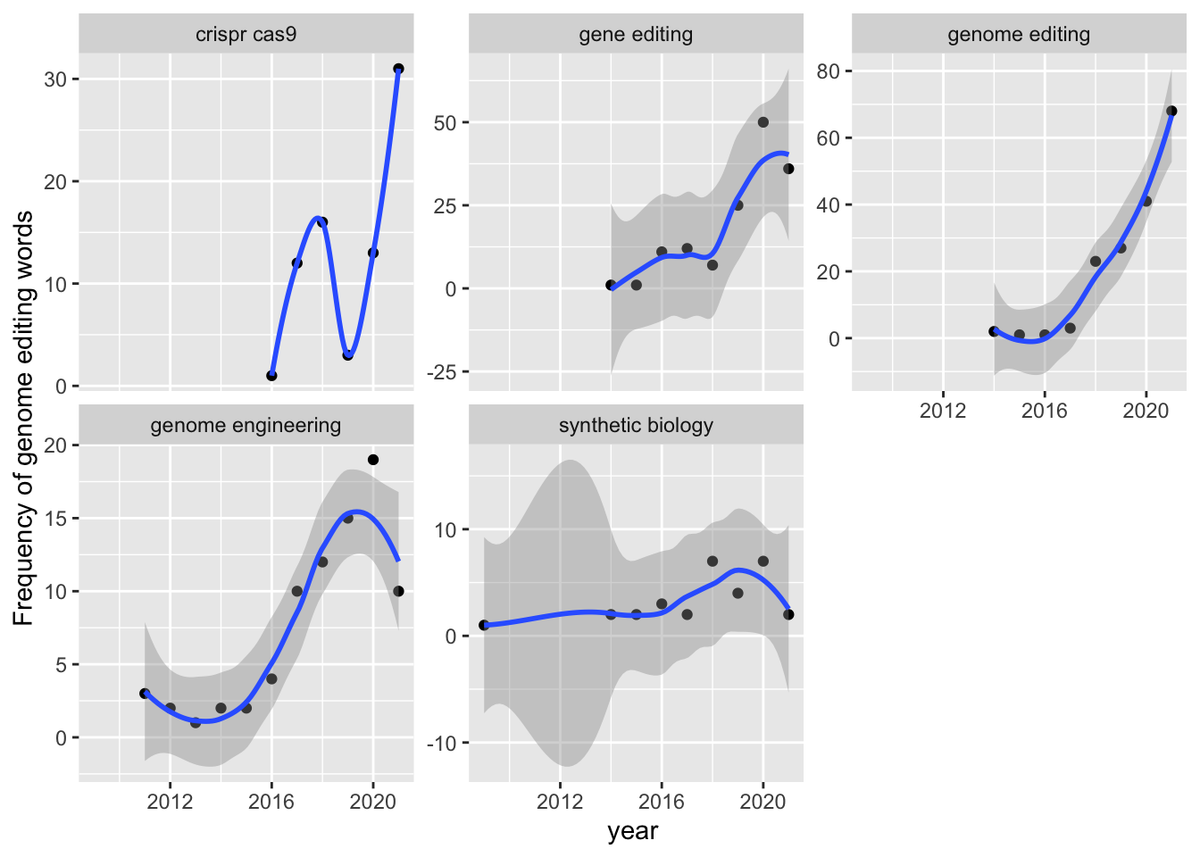
Figure 7.2: Frequency Trends for Genome Editing Terms
This example illustrates that we can readily map the emergence of terms and the frequency of their use in patent data. It is important to point out some of the limitations of this approach that will be encountered.
In the case of the present data we are working with the US patent grants data. The calculation is therefore for the emergence of terms in granted patents. As such, this does not apply to patent applications unless we explicitly include that table. A second limitation, in terms of US data, is that in the United States patent documents were only published when they were granted. It was only in 2001 that the US started publishing patent applications. Third, the data is based on publication dates. The earliest use of a term will occur in a priority application (the first filing). To map trends in the emergence of concepts over time we would therefore preferably use the priority date. In the latter case, as the actual priority document, such as as US provisional application, may not be published we are making an assumption that the terms appeared in the documents filed on the earliest priority data.
A more fundamental issue however is that our analysis of trends is restricted to the titles and abstracts of the US patent collection. For a more comprehensive and accurate treatment we would want to extend the analysis to the description and claims. This would considerably expand the size of the data we would need to work with and thus demand engagement with cloud computing and the use of tools such as Apache Spark (for parallel computing).
As such, in reality when mapping trends in the emergence of terms and in potentially seeking to forecast likely trends based on the existing data we would want to make some adjustments to this approach for patent data. Nevertheless, mapping of the emergence of terms is relatively straightforward. A simpler example on which the example above is based is available in Silge and Robinson 2017 (at pages 76 to 77), using texts from presidential inaugural speeches.
7.9 Correlation Measures
Word and phrases in a text exist in relationship to other words and phrases in the text. As we will see in the chapter on machine learning, an understanding of these relationships and methods for calculating and predicting these relationships have been fundamental to advances in Natural Language Processing in recent years.
One of the most useful of these measures in text mining is co-occurrence. That is, what words or phrases occur with other words and phrases in a text or group of texts. In the discussion above we created a data frame containing the distinctive bigrams in each text associated with genome editing.
We can take a look at the phrases linked to our target terms in Figure 7.3 below.
| patent_id | publication_number | bigram | n | tf | idf | tf_idf |
|---|---|---|---|---|---|---|
| 10000800 | US10000800B2 | oligonucleotide constructs | 3 | 0.1578947 | 10.114995 | 1.5971045 |
| 10000800 | US10000800B2 | validated sequences | 2 | 0.1052632 | 10.808142 | 1.1376992 |
| 10000800 | US10000800B2 | analysis polymorphism | 1 | 0.0526316 | 10.808142 | 0.5688496 |
| 10000800 | US10000800B2 | biology quantitative | 1 | 0.0526316 | 10.808142 | 0.5688496 |
| 10000800 | US10000800B2 | constructs sets | 1 | 0.0526316 | 10.808142 | 0.5688496 |
| 10000800 | US10000800B2 | desired rois | 1 | 0.0526316 | 10.808142 | 0.5688496 |
| 10000800 | US10000800B2 | provide validated | 1 | 0.0526316 | 10.808142 | 0.5688496 |
| 10000800 | US10000800B2 | validated rois | 1 | 0.0526316 | 10.808142 | 0.5688496 |
| 10000800 | US10000800B2 | mutation screening | 1 | 0.0526316 | 10.451467 | 0.5500772 |
| 10000800 | US10000800B2 | quantitative nucleic | 1 | 0.0526316 | 9.981464 | 0.5253402 |
| 10000800 | US10000800B2 | synthetic biology | 1 | 0.0526316 | 9.421848 | 0.4958867 |
| 10000800 | US10000800B2 | acid analysis | 1 | 0.0526316 | 7.369557 | 0.3878714 |
| 10000800 | US10000800B2 | acid constructs | 1 | 0.0526316 | 5.695294 | 0.2997523 |
| 10000800 | US10000800B2 | wide variety | 1 | 0.0526316 | 5.106266 | 0.2687509 |
| 10000800 | US10000800B2 | nucleic acid | 2 | 0.1052632 | 2.549202 | 0.2683370 |
| 10006054 | US10006054B1 | encoding genome | 1 | 0.0476190 | 11.367758 | 0.5413218 |
| 10006054 | US10006054B1 | include inserts | 1 | 0.0476190 | 11.367758 | 0.5413218 |
| 10006054 | US10006054B1 | inserts encoded | 1 | 0.0476190 | 11.367758 | 0.5413218 |
| 10006054 | US10006054B1 | ogrna targeting | 1 | 0.0476190 | 11.367758 | 0.5413218 |
| 10006054 | US10006054B1 | rna ogrna | 1 | 0.0476190 | 11.367758 | 0.5413218 |
What we are seeking to understand using this data is what are the top co-occurring terms. To do this we will cast the data into a matrix where the bigrams are mapped against each other producing a correlation value. Using the widyr package we then pull the data back into columns with the recorded value.
There are a variety of packages for calculating correlations and cooccurrences with texts. We will use udpipe package by Jan Wijffels for illustration of this approach (Wijffels 2022). The widyr package offers a pairwise_count() function that achieves the same thing in fewer steps. However, udpipe is easy to use and it also offers additional advantages such as parts of speech tagging (POS) for nouns, verbs and adjectives (Robinson 2021).
First, we calculate term frequencies for our bigrams (in practice we have these but we illustrate from scratch here) using the patent_id as the identifier and the bigram. Next, we cast the data into a matrix of the bigrams against the bigrams (dtm). This transforms our dataset containing 4,430 rows into a large and sparse matrix with 3.6 million observations (where most values are zero because there is no correlation). Then apply a correlation function (in this case Pearson’s, also known as Pearson’s R, but a range of other correlation functions are available) to obtain the correlation coefficient. Finally, the matrix is transformed back into a data.frame that drops empty (0) items in the sparse matrix. In the cooccurrence data frame term1 is the source and term2 is the target with a range of scores expressed from -0.n to 1.
library(udpipe)
dtf <- document_term_frequencies(gene_editing_tfidf, document = "patent_id", term = "bigram")

dtm <- document_term_matrix(dtf)

correlation <- dtm_cor(dtm)

cooccurrence <- as_cooccurrence(correlation)
The cooccurrence matrix contains 3.6 million rows of co-occurrences between bigrams in the dataset. We filter the dataset to “genome editing” in Figure 7.3 below in order to see the outcome for one of the terms.
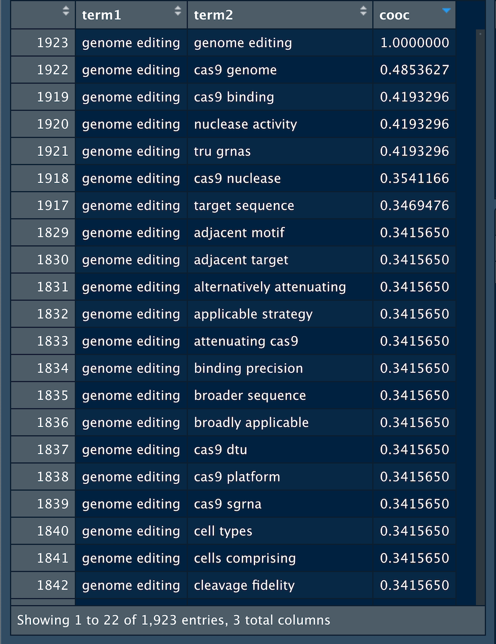
Figure 7.3: Cooccurrence Scores for Gene Editing
The cooccurrence value for the matching term (in this case “genome editing”) is always 1. Inside the actual matrix this displays on the diagonal in the centre of the matrix and gives rise to the expression “removing the diagonal” or self-reference. We can do this by filtering to keep any value that does not equal 1 as we see in Table 7.17.
| term1 | term2 | cooc |
|---|---|---|
| genome engineering | genome editing | -0.3913164 |
| genome editing | genome engineering | -0.3913164 |
| genome editing | gene editing | -0.3725150 |
| gene editing | genome editing | -0.3725150 |
| genome engineering | gene editing | -0.2669573 |
| gene editing | genome engineering | -0.2669573 |
The data from the title and abstracts using tf_idf now suggests the strong correlation between gene editing and genome engineering in our example dataset.
In common with the network visualisations discussed in the last chapter, this data can also be visualised in a network where term1 constitutes the source node, term2 the target node and cooc (or n) the weight of the edge between source and target nodes. For simplicity in presentation we will select only terms with a cooccurence score over .10 for genome editing. The code here is adapted directly from the udpipe documentation.
library(igraph)
library(ggraph)

cooccurrence_clean %>%
  filter(term1 == "genome editing") %>%
  arrange(cooc) %>%
  filter(cooc  > .10) %>%
  graph_from_data_frame() %>%
  ggraph(layout = "fr") +
  geom_edge_link(aes(width = cooc, edge_alpha = cooc), edge_colour = "pink") +
  geom_node_text(aes(label = name), col = "darkgreen", size = 2) +
  theme_graph(base_family = "Arial Narrow") +
  theme(legend.position = "none") +
  labs(title = "Genome Editing Cooccurrence Network")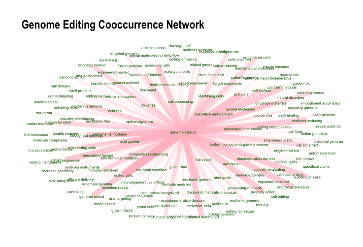
Figure 7.4: Genome Engineering Network
The visualisation of networks is a powerful tool for making decisions about how to proceed with analysis. In particular, visualisation of networks of terms is an extremely useful device when seeking directions for further analysis, for example on the use of genome editing in therapeutics or in agriculture and other applications.
The use of these methods is not confined to patent researchers with programming skills. VantagePoint from Search Technology Inc provides many of these tools out of the box and has considerable strength of allowing greater freedom and precision in interactive exploration and refinement of the data.
7.10 Conclusion
Recent years have witnessed a dramatic transformation in the availability of patent data for text mining at scale. The creation of the USPTO PatentsView Data Download service, formatted specifically for patent analysis, represents an important landmark as does the release of the full texts of EPO patent documents through Google Cloud. Other important developments include the Lens Patent API service that provides access to the full text of patent documents under a range of different plans, including free access. It remains to be seen whether WIPO will follow these developments by making the full texts of PCT documents freely available for use in patent analytics.
Growing access to data also presents challenges, such as how to download, store and update large patent datasets. A second challenge is how to transform such data from XML or JSON (from calls to APIs) into formats that can be used for analysis. Finally, analysis steps themselves require data cleaning, text mining skills, some statistical and machine learning skills. In many cases software packages in R and Python or the use of VantagePoint ease the way in creating patent analytics workflows. However, the immediate practical challenge for the patent analyst will be text mining with datasets that are either too large for memory or are unwieldy on their platforms. We close this chapter with some suggestions on ways forward.
In the preceding discussion we suggested that there is a process for working with textual data at scale. This consists of the following steps.
- Use text mining with a range of terms to identify other terms that define the universe of things you are interested in;
- Identify the relevant areas of the patent classification that the terms fit into;
- Filter the data down to the selected terms and patent classification codes;
- Use measures such as term frequency inverse document frequency to identify distinctive terms in your data either at the level of words or phrases and experiment until the set meets your needs;
- Section the data into groupings for analysis using either the IPC as a guide, groupings of terms arising from tfidf and/or use Latent Dirichlet Allocation (LDA) and similar techniques for topic modelling;
- Use experimental visualisation (such as network visualisation) along the way to test and refine your analysis.
As analysis proceeds text mining will increasingly move into matrix operations and correlation and co-occurrence measures to identify and examine clusters of terms. These operations are directed to opening the path to producing analytical outputs on your topic of interest that are meaningful to non-patent specialists. Rather than seeing the steps outlined above as obligatory it is important to recognise when and where to use particular tools. For example, it turned out that there was not much to be gained from LDA on genome editing in terms of topic modelling because the topic had already been identified. As such, identifying the appropriate tool for the task at a particular moment in the workflow is an important skill.
It is also important to recognise that analysts seeking to reproduce the steps in this Chapter will often be pushing the boundaries of their computing capacity. Here is is important to emphasise that an important principle when working with data at scale is to identify the process for reducing scale to human manageable levels as soon as is practical. It is inevitable however, that working at scale creates issues where data will not fit into memory (out of memory or oom) or processing capacity is insufficient for timely analysis. Of all the tasks involved in patent analytics, text mining and machine learning rapidly push at the boundaries of computing capacity.
The solution to compute limitation is not to buy every bigger computers but to recognise that extra capacity can be acquired in the cloud through companies such as Amazon Web Services, Google Cloud or Microsoft Azure (among many others). For example, a large Windows Server can be set up to run VantagePoint on large datasets or virtual machines for work with Python and R. For large scale parallel computing of texts services such as Databricks Apache Spark clusters can be created that will cost a few dollars an hour to run. When processing is completed data can be exported and analysis and payment for the service can stop. This ability to scale up and scale down computing capacity as required is the major flexibility offered by cloud computing services and we recommend exploring these options if you intend to work with text data at scale. Many tutorials exist on setting up virtual machines and clusters with different services.
The text mining techniques introduced in this chapter are part of a wider set of techniques that can be tailored for specific needs. However, rapid advances in machine learning in recent years are transforming natural language processing. The topics discussed in this chapter are a useful foundation for understanding these transformations. We now turn to the use of machine learning in patent analytics.